Grid-connected inverters and grid-forming control

The inverter is the heart of every solar plant and battery, and at the point of interconnection it is the only part of the plant the grid actually sees. The power electronics course covered how an inverter's switches synthesize an AC waveform. This lesson looks at the inverter from the grid's side: how it decides how much current to inject and at what angle, what limits its output, what happens when the grid is weak, and how a new class of grid-forming inverters behaves more like a voltage source than a current source.

The inverter as a controlled current source

Almost every inverter connected to the grid today is grid-following. Its control system measures the voltage at its terminals, uses a phase-locked loop (PLL) to estimate the angle and frequency of that voltage, and then regulates its output current to a reference expressed relative to that angle. A current component in phase with the voltage delivers real power; a component 90° out of phase delivers reactive power. The outer control loops set those two components from the requested real power P and reactive power Q, and a fast inner current loop, running thousands of times a second, drives the switches to make the actual current follow the reference.

In other words, a grid-following inverter behaves as a controlled current source synchronized to a voltage that something else establishes. It depends on the grid to provide a stable voltage waveform to lock onto. That is perfectly adequate on a strong grid dominated by synchronous generators, and it is why grid-following control has been the default for decades. It becomes a weakness when inverters make up a large share of the generation in an area, because there may be too little voltage-forming capability left for the PLLs to lock onto reliably.

Current limits and the capability curve

The semiconductors in an inverter are rated for a maximum current, and that current limit, not a voltage or power limit, governs everything the inverter can do. At rated voltage the current limit corresponds to the inverter's apparent power rating in kVA or MVA. When the grid voltage sags, the same current carries less power, so the available apparent power falls in proportion to voltage. At the other end, the DC side sets a separate limit on real power: a solar inverter cannot export more than its array supplies, and a battery inverter is limited by the battery's discharge rating.

import math, cmath
# 1. Capability of Birch Hill's solar inverters at the POI (4 x 2.75 MVA)
S_RATED = 11.0                                   # MVA at 1.0 pu voltage
for v in (1.05, 1.00, 0.95, 0.90):
    s = S_RATED*v                                # current-limited: S falls with voltage
    q = math.sqrt(max(s**2 - 10.0**2, 0))
    print(f"V = {v:.2f} pu: S max {s:5.2f} MVA, Q available at 10 MW = {q:4.2f} Mvar (pf {10/s if s > 10 else 1:.2f})")
# 2. Grid strength at the point of interconnection: short-circuit ratio
V = 24.94; Ssc_bus = math.sqrt(3)*V*5.62                       # MVA at the 25 kV bus
Zs = complex(0.10, 1.0)/abs(complex(0.10, 1.0))*V**2/Ssc_bus   # source impedance, X/R 10
for km in (11, 25):
    Z = Zs + complex(0.11, 0.40)*km
    Ssc = V**2/abs(Z); scr = Ssc/10.0
    print(f"POI {km:2d} km out: Ssc = {Ssc:5.1f} MVA, SCR = {scr:4.1f}  ({'strong' if scr >= 3 else 'weak'})")
# 3. Two grid-forming inverters sharing a load step by frequency droop (islanded)
P1n, P2n, m = 2.5, 5.0, 0.02          # MW ratings, 2 % droop on each unit's own rating
load = 4.2                             # MW step on the island
# f = 60(1 - m(P/Pn)) for each unit; equal frequency means P1/P1n = P2/P2n
share = load/(P1n + P2n); f = 60*(1 - m*share)
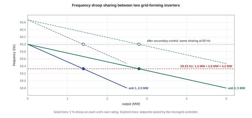
print(f"Load {load} MW: unit 1 {share*P1n:.2f} MW, unit 2 {share*P2n:.2f} MW, frequency {f:.2f} Hz")

V = 1.05 pu: S max 11.55 MVA, Q available at 10 MW = 5.78 Mvar (pf 0.87)
V = 1.00 pu: S max 11.00 MVA, Q available at 10 MW = 4.58 Mvar (pf 0.91)
V = 0.95 pu: S max 10.45 MVA, Q available at 10 MW = 3.03 Mvar (pf 0.96)
V = 0.90 pu: S max  9.90 MVA, Q available at 10 MW = 0.00 Mvar (pf 1.00)
POI 11 km out: Ssc =  87.6 MVA, SCR =  8.8  (strong)
POI 25 km out: Ssc =  48.2 MVA, SCR =  4.8  (strong)
Load 4.2 MW: unit 1 1.40 MW, unit 2 2.80 MW, frequency 59.33 Hz

The first part of the program shows what this means for Birch Hill. At nominal voltage the four inverters' 11 MVA allows 4.6 Mvar of reactive power at full real output, a power factor of about 0.91. At 1.05 pu voltage the margin grows. At 0.95 pu it shrinks to 3.0 Mvar, and at 0.90 pu the inverters can deliver 10 MW but no reactive power at all. Many plants are therefore specified with a reactive capability defined at a range of voltages, and the plant controller is set to give priority either to real or to reactive current when the two compete, a choice that standards now often specify, especially during disturbances.

Grid strength and the short-circuit ratio

The strength of the grid at a point is measured by its short-circuit capacity: the three-phase fault power available there, which is inversely proportional to the impedance between that point and the sources of the system. Planners compare it with the resource's rating to get the short-circuit ratio (SCR). A high SCR means the grid's voltage barely moves when the plant changes output. A low SCR, typically below about 3, means the plant's own current noticeably moves the voltage it is trying to follow, and grid-following controls can interact with the grid, oscillate or lose synchronism.

The program computes the SCR at Birch Hill's proposed point of interconnection. Lincoln Road's 25 kV bus has a three-phase fault level of about 243 MVA. Eleven kilometres of feeder add impedance, and the fault level at the POI falls to about 88 MVA, an SCR of 8.8 for the 10 MW plant. Even 25 km out, the SCR would still be about 4.8. Birch Hill is not weak-grid territory. The problem appears with large wind and solar plants in remote areas connected through long lines, or where many plants share the same weak point of the transmission system. For such plants, studies use detailed electromagnetic transient models rather than the simpler models used for strong grids.

Grid-forming inverters

A grid-forming inverter turns the relationship around. Instead of following an externally established voltage, it regulates its own internal voltage magnitude and angle, behaving like a voltage source behind an impedance, much as a synchronous generator does. Its output current is whatever the network draws from that voltage source, subject to the inverter's current limits. Because it sets a voltage rather than tracking one, it can energize a dead network, operate an island with no other sources, and stiffen a weak grid instead of being destabilized by it.

Several control approaches achieve grid-forming behaviour. Droop control is the simplest: the inverter lowers its frequency slightly as its real power output rises, and lowers its voltage as its reactive power output rises, mimicking the governor and voltage droops of synchronous generators. Virtual synchronous machine control adds an emulated rotating mass, so that frequency changes are smoothed by a virtual inertia constant. Other schemes, such as dispatchable virtual oscillator control, use nonlinear oscillator dynamics. In all of them, the inverter responds to a load change within the first few milliseconds, because its voltage source supplies the current immediately, rather than after its controls detect the change.

The last part of the program shows droop sharing in an island with two grid-forming inverters of 2.5 and 5 MW, each with a 2 % droop on its own rating. A 4.2 MW load is shared in proportion to the ratings, 1.4 and 2.8 MW, and the island settles at 59.33 Hz. A slower secondary controller, usually in a microgrid controller, then raises both frequency setpoints together to bring the island back to 60 Hz without changing the sharing. Lesson 12 returns to this when it builds the Birch Hill microgrid case.

Grid-forming capability is not free. To act as a voltage source the inverter must hold back headroom in current and, for real power, in its DC energy source. A solar plant producing at its maximum power point has no upward real-power headroom, so solar plants are rarely grid-forming on their own; batteries are the natural candidates. The inverter's current limit is also far below a synchronous generator's short-term overload capability, so a grid-forming inverter that hits its current limit during a fault must switch to a current-limiting mode and then recover to voltage-source behaviour afterwards without losing synchronism.

Where grid-forming is required

Grid-forming inverters are moving quickly from research to practice. Operators of systems with very high inverter shares, such as island grids and some regions with large wind and solar fleets, have begun to require or procure grid-forming capability from new battery plants. Industry groups have published functional specifications describing what grid-forming should mean in practice: the inverter should maintain an internal voltage phasor, respond to phase-angle jumps and frequency changes immediately, and provide damping. For a distribution utility like Larchmont, grid-forming matters most for microgrids and for black-start schemes, where some resource must establish voltage before anything else can connect.

Birch Hill's battery inverter, Leo finds in the datasheet, supports a grid-forming mode, although the developer plans to operate it as grid-following when connected. That combination is common: the plant follows the grid in normal operation and switches to grid-forming only if it is asked to energize or run an island. The interconnection agreement must say clearly which mode is allowed when, because an inverter that unexpectedly holds up voltage on a de-energized feeder is exactly the islanding hazard that protection must prevent.

Inverter models for studies

Utilities study inverter-based resources with models of different detail. Positive-sequence phasor models, used in load-flow and stability programs, represent the inverter's controls in simplified, averaged form and are adequate on strong grids. Generic models developed by industry working groups allow utilities to study plants before the manufacturer's specific model is available. Electromagnetic transient (EMT) models simulate the actual switching or average converter behaviour, the PLL and the protection logic at microsecond time steps; they are needed for weak grids, for control interactions and to investigate events where plants tripped unexpectedly.

Several large disturbances in North America over the past decade involved solar and wind plants that tripped or reduced output during transmission faults far away, because of PLL loss of synchronism, overly sensitive protection settings or momentary cessation of current. Investigations of those events, published by NERC and system operators, are a large part of why interconnection requirements now specify ride-through behaviour in detail and why accurate models must be submitted and validated, topics in lessons 6 and 11.