IIR filter design

An IIR filter uses feedback, and feedback buys sharpness cheaply. A fourth-order IIR high-pass filter costs about ten multiplies per sample; an FIR filter with the same magnitude response at a 48 kHz rate might need several hundred taps. The price is phase: IIR filters cannot have exactly linear phase, and their group delay varies across the band, as lesson 5 showed. For the APS-2's high-pass, A-weighting and equalizer filters, where only magnitude matters, IIR is the natural choice. This lesson covers the standard design route: choose an analog prototype (Butterworth, Chebyshev or elliptic), transform it to the required type of filter, and map it to the digital domain with the bilinear transform, prewarping the critical frequencies so that they land where they should. The lesson ends with a case where the standard route fails, the A-weighting filter at 16 kHz, and shows how to repair it.

Analog prototypes

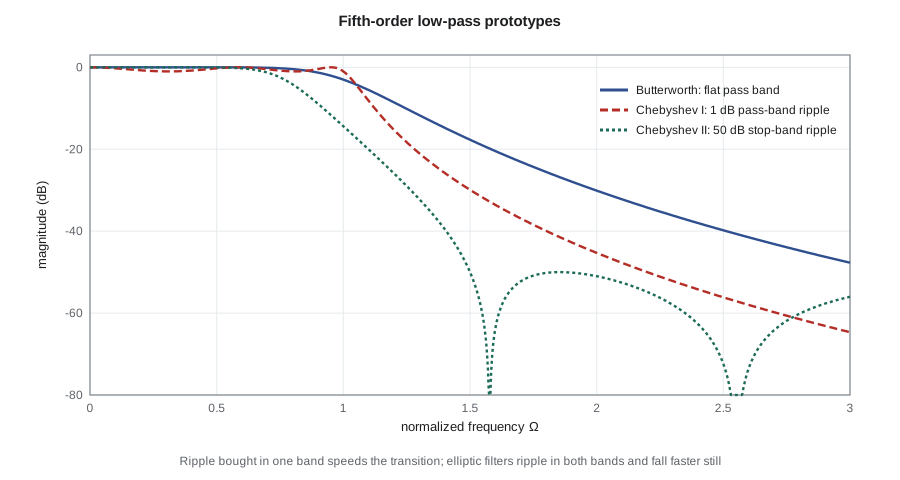
A century of analog filter theory has produced families of low-pass responses with known, optimal properties, and digital IIR design reuses them. Each is defined by the squared magnitude of its response as a function of normalized frequency Ω, with the pass-band edge at Ω = 1. The Butterworth response is maximally flat: as many derivatives as possible are zero at DC, so the pass band has no ripple and the roll-off is smooth and monotonic. The Chebyshev type I response allows equal ripple in the pass band and in return falls faster just beyond the edge. Chebyshev type II, or inverse Chebyshev, puts the ripple in the stop band instead and keeps the pass band flat. The elliptic, or Cauer, response allows ripple in both bands and gives the sharpest transition of all for a given order.

The order needed to meet a specification follows from these expressions. With pass-band ripple R_p dB and stop-band attenuation A dB at a stop-band edge Ω_s, define ε² = 10^(R_p/10) − 1 and the ratio D = (10^(A/10) − 1)/ε². The Butterworth order is n ≥ log D/(2 log Ω_s); the Chebyshev order is n ≥ arccosh √D / arccosh Ω_s. Elliptic orders need elliptic integrals, which design tools evaluate. For sharp specifications the differences are large: a Chebyshev filter typically needs about half the order of a Butterworth filter, and an elliptic filter fewer still.

Frequency transformations

Prototypes are low-pass with Ω_p = 1. Substitutions in the s-domain turn them into other shapes. Replacing s by s/Ω_c moves the edge to Ω_c. Replacing s by Ω_c/s turns a low-pass filter into a high-pass filter with edge Ω_c, mapping each pole p to Ω_c/p and adding zeros at s = 0. Replacing s by (s² + Ω₀²)/(Bs) gives a bandpass filter of bandwidth B centred at Ω₀, doubling the order. These substitutions are done in the analog domain before the bilinear transform; equivalent transformations also exist directly in the z-domain, and design tools offer both.

From s to z: impulse invariance and the bilinear transform

Two methods map an analog filter to a digital one. Impulse invariance samples the analog impulse response: each analog pole p becomes a digital pole e^(pT). The time-domain shape is preserved, but the frequency response is the analog response aliased, which ruins high-pass and band-stop filters and distorts low-pass filters near the Nyquist frequency. The bilinear transform instead substitutes a rational function of z for s. It maps the whole left half of the s-plane into the unit circle, so stable analog filters always give stable digital ones, and it maps the entire imaginary axis onto the unit circle exactly once, so there is no aliasing at all.

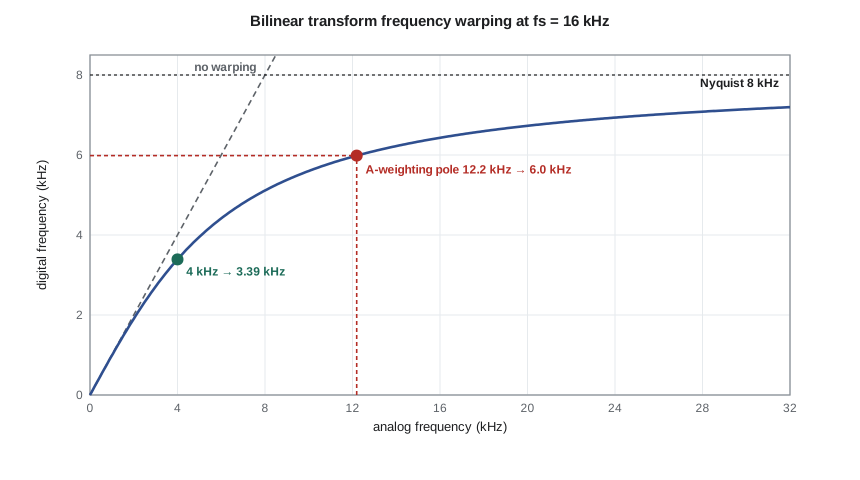
The price of avoiding aliasing is frequency warping. The infinite analog frequency axis is squeezed into −π to π, so the relationship between analog Ω and digital ω is the tangent curve above. At low frequencies, Ω ≈ ω/T and the mapping is nearly linear; as ω approaches π, Ω runs off to infinity. Any analog frequency, however high, lands below the Nyquist frequency, and an analog zero at infinity lands at z = −1, ω = π. The cure for the warping is prewarping: decide which digital frequencies matter, such as the pass-band and stop-band edges, compute the analog frequencies that the bilinear transform will map onto them, design the analog filter at those prewarped frequencies, and then transform.

Designing the APS-2 high-pass filter

The first filter in the input path removes hum and wind rumble. The microphone receiver of ELE-340 already rejects most 60 Hz common-mode hum, but some differential hum remains, and wind across the pole housing produces strong energy below 100 Hz that would otherwise dominate the headroom and confuse the echo canceller. Amara specifies a fourth-order Butterworth high-pass filter at 100 Hz, at the 48 kHz rate. At such a low frequency relative to the sample rate, prewarping barely matters, but she applies it anyway as a habit. A fourth-order Butterworth filter has two pole pairs with quality factors Q = 1/(2 sin((2k − 1)π/2n)), which for n = 4 gives 0.5412 and 1.3066, and each pair becomes one biquad.

The A-weighting filter

Sound level meters weight the spectrum to mimic human hearing at moderate levels. The A-weighting curve, standardized for sound level meters in IEC 61672, is defined by an analog filter with poles at about 20.6 Hz (double), 107.7 Hz, 737.9 Hz and 12 194 Hz (double), four zeros at the origin and a gain that makes it 0 dB at 1 kHz. It falls by about 39 dB at 31.5 Hz, 16 dB at 125 Hz, rises slightly to +1.3 dB around 2.5 kHz and falls again at high frequencies. Ambient noise limits for accessible pedestrian signals, and noise bylaws generally, are written in A-weighted decibels, dB(A), so the APS-2 level meter must apply it.

At 48 kHz, the bilinear transform of this filter is accurate: the error is under 0.05 dB up to 4 kHz and about 0.2 dB at 6.3 kHz, well within the tolerances of a sound level meter. At 16 kHz it is not. The double pole at 12.2 kHz is above the new Nyquist frequency of 8 kHz, and the bilinear transform warps it down to about 6 kHz, while the zeros it adds at z = −1 drive the response to zero at 8 kHz. The digital filter is then 0.5 dB low at 4 kHz, almost 6 dB low at 6.3 kHz and more than 20 dB low at 7.5 kHz. Prewarping cannot help, because there is no digital frequency for a pole above the Nyquist frequency to be warped to.

Amara's fix uses the fact that the APS-2 only needs the response up to about 7 kHz, where its decimation filter ends. She transforms only the low-frequency part of the filter, the poles at 20.6, 107.7 and 737.9 Hz, which the bilinear transform maps accurately. That part is a little too bright at high frequencies, because the 12.2 kHz roll-off is missing. She then adds a three-tap linear-phase FIR correction, c, 1 − 2c, c, whose gentle low-pass response replaces the missing roll-off, and chooses c to minimize the largest error between 2 and 7 kHz. The code below performs the search.

import math, cmath
fs48, fs16 = 48000, 16000
# 1. Fourth-order Butterworth high-pass at 100 Hz, 48 kHz, as two biquads
def hp_biquad(fc, Q, fs):
    K = math.tan(math.pi * fc / fs); c = 1 / (1 + K / Q + K * K)
    return [c, -2 * c, c], [1, 2 * (K * K - 1) * c, (1 - K / Q + K * K) * c]
n = 4
Qs = [1 / (2 * math.sin((2 * k - 1) * math.pi / (2 * n))) for k in range(1, n // 2 + 1)]
sos = [hp_biquad(100, Q, fs48) for Q in Qs]
def resp(sections, f, fs):
    z1 = cmath.exp(-2j * math.pi * f / fs); H = 1
    for b, a in sections:
        H *= (b[0] + b[1] * z1 + b[2] * z1 * z1) / (a[0] + a[1] * z1 + a[2] * z1 * z1)
    return H
print("Q values:", [round(q, 4) for q in Qs])
for b, a in sos:
    print("  b =", [f"{v:.8f}" for v in b], " a =", [f"{v:.8f}" for v in a])
print("high-pass:", ", ".join(f"{f} Hz {20*math.log10(abs(resp(sos, f, fs48))):6.1f} dB" for f in (30, 60, 100, 150, 1000)))
# 2. Orders for 1 dB above 150 Hz and 30 dB at 60 Hz
e2 = 10 ** 0.1 - 1; D = (10 ** 3 - 1) / e2; Ws = 150 / 60
print(f"orders: Butterworth {math.log10(D)/(2*math.log10(Ws)):.2f}, Chebyshev {math.acosh(math.sqrt(D))/math.acosh(Ws):.2f}")
# 3. A-weighting by the bilinear transform, and the 16 kHz repair
f1, f2, f3, f4 = 20.598997, 107.65265, 737.86223, 12194.217
w = lambda f: 2 * math.pi * f
def analog(f):
    s = 1j * w(f)
    return s ** 4 / ((s + w(f1)) ** 2 * (s + w(f2)) * (s + w(f3)) * (s + w(f4)) ** 2)
def digital(fs, include_hf):
    def H(f):
        z1 = cmath.exp(-2j * math.pi * f / fs); s = 2 * fs * (1 - z1) / (1 + z1)
        h = s ** 4 / ((s + w(f1)) ** 2 * (s + w(f2)) * (s + w(f3)))
        return h / (s + w(f4)) ** 2 if include_hf else h
    return H
def db_rel(H, f): return 20 * math.log10(abs(H(f)) / abs(H(1000)))
freqs = (125, 1000, 2000, 4000, 6300, 7500)
print("A-weighting (analog):", ", ".join(f"{f} Hz {db_rel(analog, f):+.1f}" for f in freqs))
for fs in (fs48, fs16):
    H = digital(fs, True)
    print(f"bilinear at {fs//1000} kHz, error dB:", ", ".join(f"{db_rel(H, f) - db_rel(analog, f):+.2f}" for f in freqs))
Hlow = digital(fs16, False)
def fir_db(c, f):
    return 20 * math.log10(abs(1 - 2 * c + 2 * c * math.cos(2 * math.pi * f / fs16)) / abs(1 - 2 * c + 2 * c * math.cos(2 * math.pi * 1000 / fs16)))
fit_f = (2000, 3150, 4000, 5000, 6300, 7000)
best = min(((max(abs(db_rel(Hlow, f) + fir_db(c, f) - db_rel(analog, f)) for f in fit_f), c) for c in [k / 2000 for k in range(200)]))
c = best[1]
print(f"repaired 16 kHz design: c = {c:.4f}, worst error 2-7 kHz {best[0]:.2f} dB")
print("repaired error dB:", ", ".join(f"{db_rel(Hlow, f) + fir_db(c, f) - db_rel(analog, f):+.2f}" for f in freqs))

Q values: [1.3066, 0.5412]
  b = ['0.99497317', '-1.98994635', '0.99497317']  a = ['1.00000000', '-1.98986110', '0.99003159']
  b = ['0.98800896', '-1.97601793', '0.98800896']  a = ['1.00000000', '-1.97593328', '0.97610258']
high-pass: 30 Hz  -41.8 dB, 60 Hz  -17.8 dB, 100 Hz   -3.0 dB, 150 Hz   -0.2 dB, 1000 Hz   -0.0 dB
orders: Butterworth 4.51, Chebyshev 3.08
A-weighting (analog): 125 Hz -16.2, 1000 Hz +0.0, 2000 Hz +1.2, 4000 Hz +1.0, 6300 Hz -0.1, 7500 Hz -0.8
bilinear at 48 kHz, error dB: -0.00, +0.00, -0.00, -0.04, -0.22, -0.43
bilinear at 16 kHz, error dB: -0.04, +0.00, -0.01, -0.49, -5.72, -22.78
repaired 16 kHz design: c = 0.0605, worst error 2-7 kHz 0.20 dB
repaired error dB: -0.02, +0.00, -0.05, -0.19, -0.03, +0.43

The high-pass filter comes out as two biquads with all their coefficients printed, ready for lesson 10 to quantize. Its response is −3 dB at 100 Hz as designed, about −18 dB at 60 Hz and −42 dB at 30 Hz. The A-weighting results confirm the analysis. At 48 kHz the bilinear design is excellent. At 16 kHz it is unusable above about 4 kHz. The repaired design, the low-frequency sections plus the three-tap correction with c ≈ 0.06, stays within about ±0.2 dB from 2 to 7 kHz and matches the low-frequency end, which is set by the accurately mapped poles, to within a few hundredths of a decibel at 125 Hz. That is comfortably inside sound level meter tolerances over the range the APS-2 measures, and it costs only two more multiplies per sample.

Practical points

Four habits make IIR design reliable. Always implement a high-order IIR filter as a cascade of second-order sections, never as one high-order difference equation; lesson 10 shows why. Pair each pole pair with the nearest zero pair and order the sections from the lowest to the highest Q, or in the order recommended by the design tool, to keep internal signal levels under control. Normalize the gain of each section so that no section amplifies a signal enough to overflow. And verify the final digital response numerically against the specification and, where one exists, against the analog reference, at the actual sample rate, because the bilinear transform can surprise anyone who works near the Nyquist frequency.