
CMPUT-415 · Lesson 11 of 12 · 37 min
Optimization and data-flow analysis
An optimizer transforms a program into an equivalent one that is better by some measure: faster, smaller or more energy-efficient. The word is a misnomer, since compilers rarely produce truly optimal code, but the improvements are large: on typical programs, compiling with -O2 rather than -O0 often makes code two to five times faster. Every optimization rests on an analysis that proves the transformation safe. Constant propagation needs to know that a variable always holds the same value at a point; dead code elimination needs to know that a value is never used; moving code out of a loop needs to know that it computes the same thing on every iteration. This lesson presents the classic optimizations and the general framework, data-flow analysis, used to justify them.
Where optimizations apply
Optimizations are classified by scope. Local optimizations work within a single basic block, where control flow is trivial. Global (intraprocedural) optimizations work on a whole function's control-flow graph. Interprocedural optimizations work across functions, using the call graph: inlining, which replaces a call with the body of the called function, is the single most important of these, because it removes call overhead and, more importantly, exposes the callee's code to every other optimization in the context of its caller. Link-time optimization (LTO) lets GCC and LLVM optimize across separately compiled files by deferring code generation until link time. Loop optimizations target the code where programs spend most of their time.
| Optimization | What it does | Required analysis |
|---|---|---|
| Constant folding | Evaluates operations on constants at compile time | None (local) |
| Constant propagation | Replaces variables known to hold constants by the constants | Reaching definitions or SSA |
| Copy propagation | Replaces y by x after y = x | Reaching copies |
| Common subexpression elimination | Reuses an already computed value | Available expressions or value numbering |
| Dead code elimination | Removes computations whose results are never used | Liveness |
| Unreachable code elimination | Removes blocks no path reaches | CFG reachability, constant branches |
| Loop-invariant code motion | Moves computations that do not change out of loops | Reaching definitions, dominators |
| Strength reduction | Replaces expensive operations by cheaper ones, such as multiply by add | Induction variable analysis |
| Inlining | Replaces a call with the callee's body | Call graph, cost model |
| Vectorization | Uses SIMD instructions for several loop iterations at once | Dependence analysis |
Local optimizations
Within a block, a single forward pass can do a great deal. Constant folding evaluates expressions whose operands are constants. Constant and copy propagation replace uses of a variable by the constant or variable it was set to. Algebraic simplification applies identities such as x × 1 = x and x − x = 0 (with care: these identities hold for integers but not always for floating point, where x − x is NaN when x is infinite). Common subexpression elimination (CSE) notices that an expression has already been computed with the same operands, and reuses the earlier result; local value numbering, which gives each distinct value a number and keys a table on the operator and operand numbers, implements this efficiently. A backward pass then performs dead code elimination, deleting instructions whose results are never used. The optimizations enable one another, so they are repeated until nothing changes.
# Local optimization of one basic block: constant folding and propagation,
# copy propagation, algebraic simplification, common subexpression
# elimination, then dead code elimination. Repeat until nothing changes.
import operator as op
OPS = {"+": op.add, "-": op.sub, "*": op.mul, "/": op.floordiv}
BLOCK = [("t1", "=", "4"), ("t2", "*", "t1", "2"), ("t3", "+", "x", "t2"),
         ("t4", "=", "t3"), ("t5", "*", "y", "1"), ("t6", "+", "x", "t2"),
         ("t7", "-", "t6", "t4"), ("t8", "+", "t5", "t7"), ("z", "=", "t8")]
LIVE_OUT = {"z"}
def is_const(a): return a.lstrip("-").isdigit()
def show(block): return "; ".join(f"{d} = {a[0]}" if o == "=" else f"{d} = {a[0]} {o} {a[1]}" for d, o, *a in block)
def one_pass(block):
    env, exprs, out = {}, {}, []
    for d, o, *args in block:
        args = [env.get(a, a) for a in args]                      # propagate constants and copies
        if o != "=" and all(is_const(a) for a in args):            # fold
            o, args = "=", [str(OPS[o](int(args[0]), int(args[1])))]
        if o == "*" and "1" in args: o, args = "=", [args[0] if args[1] == "1" else args[1]]
        if o == "+" and "0" in args: o, args = "=", [args[0] if args[1] == "0" else args[1]]
        if o == "-" and args[0] == args[1]: o, args = "=", ["0"]
        key = (o, *args)
        if o != "=" and key in exprs: o, args = "=", [exprs[key]]   # CSE: reuse earlier result
        elif o != "=": exprs[key] = d
        if o == "=": env[d] = args[0]                              # d is now a copy or a constant
        out.append((d, o, *args))
    return out
def dce(block):
    live, kept = set(LIVE_OUT), []
    for d, o, *args in reversed(block):
        if d in live: kept.append((d, o, *args)); live = (live - {d}) | {a for a in args if not is_const(a)}
    return list(reversed(kept))
b = BLOCK; print("before:", show(b))
for n in range(1, 5):
    nb = dce(one_pass(b))
    print(f"pass {n}: ", show(nb))
    if nb == b: break
b = nbbefore: t1 = 4; t2 = t1 * 2; t3 = x + t2; t4 = t3; t5 = y * 1; t6 = x + t2; t7 = t6 - t4; t8 = t5 + t7; z = t8 pass 1: z = y pass 2: z = y
Nine instructions shrink to one. Folding turns t1 × 2 into 8; CSE recognizes that t6 computes the same x + 8 as t3; t6 − t4 becomes t3 − t3, which simplifies to 0; y × 1 becomes y; and once the chain of copies is propagated, everything except z = y is dead. No single optimization achieves this, but together, repeated, they discover that the block merely copies y into z. In SSA form these optimizations are simpler still, because each name has one definition, and LLVM's instcombine and GVN passes perform them on whole functions.
Data-flow analysis
Global optimization needs facts that hold at points in the CFG, regardless of which path reached them. Data-flow analysis computes such facts with a uniform method, introduced by Gary Kildall in 1973 and developed by Frances Allen, John Cocke, Jeffrey Ullman and others. For each block, a transfer function says how the block changes the facts: facts flowing in are modified by what the block generates (GEN) and destroys (KILL), giving OUT = GEN ∪ (IN − KILL) for a forward problem. At a join, a meet operator combines the facts arriving from different predecessors: union for may analyses, where a fact holds if it holds along some path, and intersection for must analyses, where it must hold along all paths. Backward problems, such as liveness, run the same scheme against the direction of control flow.
| Analysis | Direction | Meet | Facts | Used for |
|---|---|---|---|---|
| Reaching definitions | Forward | Union (may) | Which assignments may reach a point | Constant propagation, def-use chains |
| Available expressions | Forward | Intersection (must) | Expressions computed on every path and not since changed | Global CSE |
| Live variables | Backward | Union (may) | Variables whose values may be used later | Register allocation, dead code elimination |
| Very busy expressions | Backward | Intersection (must) | Expressions evaluated on every path before their operands change | Code hoisting |
The equations are solved by iteration. Start with every block's facts at the most optimistic value (the empty set for may analyses, everything for must analyses, except at the entry or exit), then repeatedly recompute each block's IN and OUT from its neighbours until nothing changes. A worklist makes this efficient: only blocks whose inputs changed are recomputed. Visiting blocks in reverse postorder for forward problems, and postorder for backward ones, usually converges in a few passes. Because sets are represented as bit vectors with one bit per definition, expression or variable, each transfer function is a handful of bitwise operations on machine words, which is why these are called bit-vector problems.
# A generic iterative data-flow solver, instantiated for reaching definitions
# (forward, union) and live variables (backward, union) on the summing loop.
BLOCKS = {   # block: list of (definition label or None, defined var, used vars)
    "B0": [("d1", "s", []), ("d2", "i", [])],
    "B1": [(None, None, ["i", "n"])],
    "B2": [("d3", "t", ["a", "i"]), (None, None, ["t"])],
    "B3": [("d4", "s", ["s", "t"])],
    "B4": [("d5", "i", ["i"])],
    "B5": [(None, None, ["s"])]}
SUCC = {"B0": ["B1"], "B1": ["B2", "B5"], "B2": ["B3", "B4"], "B3": ["B4"], "B4": ["B1"], "B5": []}
PRED = {b: [a for a in SUCC if b in SUCC[a]] for b in SUCC}
def solve(direction, gen, kill, entry=frozenset()):
    IN = {b: set() for b in BLOCKS}; OUT = {b: set() for b in BLOCKS}
    work, steps = list(BLOCKS), 0
    while work:
        b = work.pop(0); steps += 1
        if direction == "forward":
            IN[b] = set().union(*(OUT[p] for p in PRED[b])) if PRED[b] else set(entry)
            new = gen[b] | (IN[b] - kill[b])
            if new != OUT[b]: OUT[b] = new; work += [s for s in SUCC[b] if s not in work]
        else:
            OUT[b] = set().union(*(IN[s] for s in SUCC[b])) if SUCC[b] else set(entry)
            new = gen[b] | (OUT[b] - kill[b])
            if new != IN[b]: IN[b] = new; work += [p for p in PRED[b] if p not in work]
    return IN, OUT, steps
# Reaching definitions: GEN = definitions made in the block (last one per var), KILL = other defs of those vars
defs_of = {}
for b, ins in BLOCKS.items():
    for lab, var, _ in ins:
        if lab: defs_of.setdefault(var, set()).add(lab)
gen, kill = {}, {}
for b, ins in BLOCKS.items():
    g, k = set(), set()
    for lab, var, _ in ins:
        if lab: g = {x for x in g if x not in defs_of[var]} | {lab}; k |= defs_of[var] - {lab}
    gen[b], kill[b] = g, k
IN, OUT, steps = solve("forward", gen, kill)
print(f"reaching definitions ({steps} block visits):")
for b in BLOCKS: print(f"  {b}: in {sorted(IN[b])}  out {sorted(OUT[b])}")
# Live variables: GEN = upward-exposed uses (USE), KILL = variables defined (DEF)
use, deff = {}, {}
for b, ins in BLOCKS.items():
    u, d = set(), set()
    for lab, var, used in ins:
        u |= {x for x in used if x not in d}
        if var: d.add(var)
    use[b], deff[b] = u, d
IN, OUT, steps = solve("backward", use, deff)
print(f"live variables ({steps} block visits):")
for b in BLOCKS: print(f" {b}: live in {sorted(IN[b])} live out {sorted(OUT[b])}")reaching definitions (11 block visits): B0: in [] out ['d1', 'd2'] B1: in ['d1', 'd2', 'd3', 'd4', 'd5'] out ['d1', 'd2', 'd3', 'd4', 'd5'] B2: in ['d1', 'd2', 'd3', 'd4', 'd5'] out ['d1', 'd2', 'd3', 'd4', 'd5'] B3: in ['d1', 'd2', 'd3', 'd4', 'd5'] out ['d2', 'd3', 'd4', 'd5'] B4: in ['d1', 'd2', 'd3', 'd4', 'd5'] out ['d1', 'd3', 'd4', 'd5'] B5: in ['d1', 'd2', 'd3', 'd4', 'd5'] out ['d1', 'd2', 'd3', 'd4', 'd5'] live variables (16 block visits): B0: live in ['a', 'n'] live out ['a', 'i', 'n', 's'] B1: live in ['a', 'i', 'n', 's'] live out ['a', 'i', 'n', 's'] B2: live in ['a', 'i', 'n', 's'] live out ['a', 'i', 'n', 's', 't'] B3: live in ['a', 'i', 'n', 's', 't'] live out ['a', 'i', 'n', 's'] B4: live in ['a', 'i', 'n', 's'] live out ['a', 'i', 'n', 's'] B5: live in ['s'] live out []
The results are worth reading against the CFG of lesson 8. Both definitions of s, d1 from before the loop and d4 from the loop body, reach the loop header B1 and the exit B5, which is why the SSA form needed a φ for s there. In the liveness results, a and n are live throughout the loop, because they are used on every iteration; t is live only between its definition in B2 and its last use in B3; and nothing is live into B0 except the parameters a and n. Liveness at block boundaries is exactly what the register allocator of lesson 10 needs, and pruned SSA uses it to avoid placing φ functions for dead variables such as t.
Lattices and why iteration terminates
Why does the iteration always stop, and why is the answer right? The theory, due to Kildall and refined by John Kam and Jeffrey Ullman (1976 to 1977), casts data-flow facts as elements of a lattice: a partially ordered set in which every pair of elements has a greatest lower bound, the meet. For a may analysis over sets, the order is ⊇ and the meet is union. Transfer functions are monotone: more input facts never yield fewer output facts. If the lattice has finite height, meaning there is no infinite descending chain, then each block's value can change only finitely many times, so iteration terminates. It reaches the maximal fixed point, the best solution consistent with the equations. When transfer functions are also distributive over the meet, as they are for the four bit-vector problems, this coincides with the meet-over-all-paths solution, the ideal answer obtained by considering every path separately.
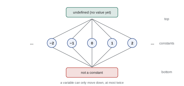
Constant propagation shows the framework beyond sets. Each variable's fact is an element of the flat lattice in the figure: undefined (no value seen yet), a particular constant, or not-a-constant. The meet of two different constants is not-a-constant; the meet of undefined with c is c. The lattice has height 3, so each variable changes at most twice and iteration terminates quickly, even though there are infinitely many constants. This analysis is not distributive: the maximal fixed point can be less precise than considering paths separately, for example when x + y is constant only because x and y vary together. Wegman and Zadeck's sparse conditional constant propagation runs this lattice over SSA def-use edges, tracking executable edges too, so that branches on constants prune unreachable code during the analysis.
Loop optimizations
Programs spend most of their time in loops, and loop optimizations are among the most profitable. Loops are identified from back edges (lesson 7): a natural loop of a back edge n → h consists of h and every block that can reach n without passing through h; h, the header, dominates the whole loop. Loop-invariant code motion moves computations whose operands do not change within the loop, such as x × y in a[i] = a[i] + x × y, into a preheader block that runs once before the loop; the analysis must check that the operands' reaching definitions are all outside the loop, and the motion must not introduce exceptions or side effects on paths where the computation would not have happened. Induction variable analysis finds variables that change by a constant amount each iteration, such as i, and expressions that are linear in them, such as the address a + 4i. Strength reduction then replaces the multiplication in the address by a pointer that is incremented by 4, and induction variable elimination may remove i altogether by rewriting the loop test in terms of the pointer.
cat scale.c
clang --target=riscv64 -O2 -fno-vectorize -fno-unroll-loops -S scale.c -o - | sed -n "/^scale:/,/ret/p" | grep -v "^\s\+\." | grep -v "^#"$ cat scale.c
void scale(int *a, int n, int x, int y) {
for (int i = 0; i < n; i++)
a[i] = a[i] + x * y;
}
$ clang --target=riscv64 -O2 -fno-vectorize -fno-unroll-loops -S scale.c -o - | sed -n "/^scale:/,/ret/p" | grep -v "^\s\+\." | grep -v "^#"
scale: # @scale
blez a1, .LBB0_3
mul a2, a3, a2
slli a1, a1, 2
add a1, a1, a0
.LBB0_2: # =>This Inner Loop Header: Depth=1
lw a3, 0(a0)
add a3, a3, a2
sw a3, 0(a0)
addi a0, a0, 4
bne a0, a1, .LBB0_2
.LBB0_3:
retThe RISC-V code shows all three loop optimizations. The multiplication mul a2, a3, a2 happens once, before the loop. Inside the loop there is no multiplication by 4 and no index i at all: a0 is a pointer incremented by 4 each iteration, and the loop ends when it reaches a1, the address one past the last element, computed before the loop as a + 4n. The loop body is five instructions. With vectorization enabled and a vector-capable target, LLVM would go further and process several elements per instruction using the RISC-V vector extension.
Further loop transformations restructure iteration. Loop unrolling replicates the body to reduce branch overhead and expose more instructions to scheduling. Loop interchange swaps nested loops so that inner iterations walk memory sequentially, which can improve cache behaviour dramatically for arrays. Fusion and fission combine or split loops; tiling breaks iteration spaces into blocks that fit in cache. These require dependence analysis, which determines whether two array accesses in different iterations can touch the same element, and polyhedral compilation, available in GCC (Graphite) and LLVM (Polly), models nested loops as integer polyhedra to choose such transformations systematically.
Inlining and the pass pipeline
Inlining deserves special mention because it amplifies everything else. After inlining, constants passed as arguments propagate into the callee's body, branches on them fold away, and loops in the callee can be optimized together with code around the call. The cost is code growth, which can hurt instruction-cache performance, so compilers use cost models: small functions and functions called once are inlined eagerly, large ones rarely. Profile-guided optimization (PGO), which compiles once with instrumentation, runs representative inputs, and recompiles with the measured branch and call frequencies, lets the compiler inline and lay out code where it matters; JIT compilers do this automatically. LLVM's -O2 pipeline runs on the order of a hundred passes, interleaving simplification (instcombine, SCCP, dead code elimination, CFG simplification), inlining over the call graph bottom up, loop passes, and vectorization, with clean-up passes between them, because each transformation creates new opportunities for the others.
Correctness and undefined behaviour
An optimization is correct only if it preserves the program's observable behaviour, and the precise meaning of observable is set by the language. In C and C++, programs with undefined behaviour, such as signed integer overflow, out-of-bounds accesses or reads of uninitialized variables, have no meaning at all, so the optimizer may assume they never occur. This is what allows Clang to transform i <= n loops assuming i never wraps around, and it is why optimizers sometimes delete null-pointer checks that appear after a dereference: having dereferenced the pointer, the program has promised it was not null. Such reasoning is valid by the language rules but surprising to programmers, and it has caused real security problems, which is why flags such as -fwrapv and -fno-delete-null-pointer-checks exist and why languages like Rust and Java define behaviour that C leaves undefined. Lesson 12 discusses how compilers themselves are tested and verified.
Worked examples
Worked problem
Folding and propagation
Optimize the block a = 3; b = a + 2; c = b * a; d = c - c; e = d + x.
Show solution
- Propagate a = 3 and fold: b = 5, then c = 15.
- d = c − c simplifies to 0, so e = 0 + x simplifies to e = x.
- If only e is live afterwards, a, b, c and d are dead and are removed.
Answer: The block becomes e = x.
Worked problem
Live variables by hand
In a block x = a + b; y = x * c; return y, which variables are live on entry?
Show solution
- Work backwards. Before return y: {y}.
- Before y = x * c: remove y, add x and c, giving {x, c}.
- Before x = a + b: remove x, add a and b, giving {a, b, c}.
Answer: a, b and c are live on entry; x and y are not.
Worked problem
Is it loop-invariant?
In while i < n { t = k * 4; i = i + t; }, is t = k * 4 invariant, and can it be hoisted?
Show solution
- k is not assigned in the loop, so all definitions of k reaching the statement are outside: the computation is invariant.
- Hoisting to the preheader would execute it even if the loop runs zero times; multiplication cannot fail, so this is safe.
- After hoisting, t is assigned once before the loop and only read inside it.
Answer: Yes; it can be moved to the preheader. A division by k would need care, because it could fault when the loop body never runs.
Common mistakes
MistakeApply x − x = 0 to floating-point values.
InsteadIt fails for infinities and NaN; floating-point identities need fast-math permission.
MistakeRun each optimization once.
InsteadOptimizations enable one another, so pipelines repeat and interleave them.
MistakeUse union as the meet for available expressions.
InsteadAvailable expressions is a must analysis; the meet is intersection.
MistakeHoist any invariant computation out of a loop.
InsteadCheck it cannot fault or have side effects on paths where it would not have run.
MistakeTreat code relying on signed overflow as safe under optimization.
InsteadSigned overflow is undefined in C; the optimizer may assume it never happens.
Summary and key terms
- Optimizations transform programs into faster or smaller equivalents; each relies on an analysis proving it safe.
- Local optimizations such as folding, propagation, CSE and dead code elimination work within blocks and enable one another.
- Data-flow analysis computes facts at CFG points with transfer functions and a meet operator, forward or backward, may or must.
- Iterative worklist algorithms converge because transfer functions are monotone and lattices have finite height.
- Reaching definitions, available expressions, live variables and very busy expressions are the classic bit-vector problems.
- Loop optimizations include invariant code motion, strength reduction, induction variable elimination, unrolling and interchange.
- Inlining and profile guidance multiply the benefits; correctness depends on the language's precise semantics, including undefined behaviour.
- Constant folding
- Evaluating operations on constant operands at compile time.
- Common subexpression elimination
- Reusing a previously computed value instead of recomputing it.
- Dead code elimination
- Removing computations whose results are never used.
- Data-flow analysis
- Computing facts that hold at program points over all paths, by solving equations on the CFG.
- Transfer function
- A function describing how a block changes the data-flow facts.
- Meet operator
- The operation combining facts at a join, such as union or intersection.
- Reaching definitions
- The assignments whose values may reach a program point.
- Live variable
- A variable whose current value may be used later.
- Lattice
- A partially ordered set with meets, used to model data-flow facts.
- Loop-invariant code motion
- Moving computations that do not change within a loop to before it.
Practice problems
Work each problem on paper first, then reveal the answer to check.
What does constant folding do to 6 * 7?
Show answer
Replaces it with 42 at compile time.
Which analysis does dead code elimination need?
Show answer
Liveness.
Is reaching definitions a forward or backward problem?
Show answer
Forward.
What is the meet operator for a must analysis?
Show answer
Intersection.
Why are the classic analyses called bit-vector problems?
Show answer
Their facts are sets represented as bit vectors, so transfer functions are bitwise operations.
In the data-flow output, which definitions of s reach B5?
Show answer
d1 and d4.
What property of transfer functions guarantees termination together with finite height?
Show answer
Monotonicity.
What does strength reduction replace in a[i] inside a loop?
Show answer
The multiplication i × 4 in the address, by a pointer incremented each iteration.
What is a loop preheader?
Show answer
A block inserted before the header that runs once before the loop, where invariant code is placed.
Why is inlining so valuable?
Show answer
It removes call overhead and exposes the callee's code to optimization in the caller's context.
Lesson quiz · 5 questions
Score 60% or more to complete this lesson.
Create a free account to save your progress, take quizzes and earn a certificate.