
CMP-330 · Lesson 7 of 12 · 35 min
The transport layer II: TCP
TCP, the Transmission Control Protocol, carries most of the internet's traffic, including web pages over HTTP/1.1 and HTTP/2, email, file transfers and remote logins. Defined in RFC 793 in 1981 and consolidated with forty years of updates in RFC 9293 in 2022, it provides a reliable, in-order, full-duplex byte stream between two processes, with flow control so the sender does not overwhelm the receiver and congestion control so senders together do not overwhelm the network. This lesson covers TCP's segment format, connection setup and teardown, how it achieves reliability with the mechanisms of lesson 6, how it estimates timeouts, and how its congestion control evolved from Reno to CUBIC and BBR. We end by comparing TCP with QUIC.
The TCP segment
A TCP segment has a header of at least 20 bytes. TCP numbers bytes, not segments: the sequence number is the position in the byte stream of the segment's first data byte, and the acknowledgement number is the next byte the receiver expects, a cumulative acknowledgement. Six commonly discussed flag bits mark special segments: SYN to open a connection, FIN to close one direction, RST to abort, ACK when the acknowledgement field is valid, PSH to ask the receiver to deliver data promptly, and URG (rarely used). The receive window field advertises how many more bytes the receiver can buffer. Options include the maximum segment size (MSS), window scaling, timestamps and selective acknowledgements.
| Field | Bits | Purpose |
|---|---|---|
| Source and destination ports | 16 each | Identify the sockets at each end |
| Sequence number | 32 | Byte-stream position of the first data byte in this segment |
| Acknowledgement number | 32 | Next byte expected from the other side (cumulative) |
| Data offset | 4 | Header length in 32-bit words, to find the start of the data |
| Flags | 8 (of 12 reserved and flag bits) | CWR, ECE, URG, ACK, PSH, RST, SYN, FIN |
| Receive window | 16 | Bytes the receiver can accept, scaled by the window scale option |
| Checksum | 16 | Internet checksum over a pseudo-header, header and data |
| Urgent pointer | 16 | Rarely used |
| Options | 0 to 320 | MSS, window scale, SACK permitted and blocks, timestamps |
Opening and closing a connection
TCP is connection-oriented: both ends must agree to communicate and set up state first. The three-way handshake does this. The client sends a SYN segment carrying a randomly chosen initial sequence number, \(x\). The server replies with a SYN-ACK carrying its own initial sequence number \(y\) and acknowledging \(x + 1\). The client replies with an ACK acknowledging \(y + 1\), and may include data in it. Random initial sequence numbers protect against old segments from an earlier connection being mistaken for new ones and make it harder for an attacker to inject forged segments. The handshake costs one round trip before data can flow; TCP Fast Open (RFC 7413) allows data in the SYN for repeat visitors, but middleboxes interfere with it and it is not widely used.
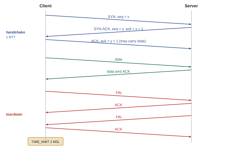
Closing is a four-step exchange because each direction closes separately: one side sends FIN, the other acknowledges it, and later sends its own FIN, which is acknowledged in turn. The side that closes first enters the TIME_WAIT state and waits for twice the maximum segment lifetime, typically 60 seconds in practice, before releasing the connection. TIME_WAIT ensures that a lost final ACK can be resent and that stray segments from the old connection die out before the same four values are reused. The program below walks through the states each side passes through.
# A tiny model of TCP connection states for a client that opens and then closes first
transitions = {
    ("CLOSED", "app connect / send SYN"): "SYN_SENT",
    ("SYN_SENT", "recv SYN+ACK / send ACK"): "ESTABLISHED",
    ("ESTABLISHED", "app close / send FIN"): "FIN_WAIT_1",
    ("FIN_WAIT_1", "recv ACK"): "FIN_WAIT_2",
    ("FIN_WAIT_2", "recv FIN / send ACK"): "TIME_WAIT",
    ("TIME_WAIT", "wait 2 x MSL"): "CLOSED",
}
server = {
    ("LISTEN", "recv SYN / send SYN+ACK"): "SYN_RCVD",
    ("SYN_RCVD", "recv ACK"): "ESTABLISHED",
    ("ESTABLISHED", "recv FIN / send ACK"): "CLOSE_WAIT",
    ("CLOSE_WAIT", "app close / send FIN"): "LAST_ACK",
    ("LAST_ACK", "recv ACK"): "CLOSED",
}
for title, table, state in (("client", transitions, "CLOSED"), ("server", server, "LISTEN")):
    print(title)
    for (s, event), nxt in table.items():
        assert s == state, (s, state)
        print(f"  {state:12s} --[{event}]--> {nxt}")
state = nxtclient CLOSED --[app connect / send SYN]--> SYN_SENT SYN_SENT --[recv SYN+ACK / send ACK]--> ESTABLISHED ESTABLISHED --[app close / send FIN]--> FIN_WAIT_1 FIN_WAIT_1 --[recv ACK]--> FIN_WAIT_2 FIN_WAIT_2 --[recv FIN / send ACK]--> TIME_WAIT TIME_WAIT --[wait 2 x MSL]--> CLOSED server LISTEN --[recv SYN / send SYN+ACK]--> SYN_RCVD SYN_RCVD --[recv ACK]--> ESTABLISHED ESTABLISHED --[recv FIN / send ACK]--> CLOSE_WAIT CLOSE_WAIT --[app close / send FIN]--> LAST_ACK LAST_ACK --[recv ACK]--> CLOSED
The handshake has a famous weakness. A server that allocates state for every SYN can be exhausted by a flood of forged SYNs that never complete, a SYN flood. SYN cookies defend against it by encoding the connection's parameters into the server's initial sequence number, so the server keeps no state until the final ACK proves the client is real. CISSP-113 lesson 10 covers such attacks.
Reliability in TCP
TCP combines the mechanisms of lesson 6. Acknowledgements are cumulative, like Go-Back-N, but receivers buffer out-of-order segments, and with the SACK option (RFC 2018) they report exactly which blocks arrived, so senders retransmit only the missing data, like Selective Repeat. Receivers may delay acknowledgements briefly, acknowledging every second full segment or after a short timeout, to halve the number of ACKs. A sender retransmits in two situations. When the retransmission timer expires, it resends the oldest unacknowledged segment. And when it receives three duplicate acknowledgements, each repeating the same acknowledgement number because later segments arrived after a gap, it assumes the segment at the gap was lost and retransmits it at once, without waiting for the timer. This fast retransmit recovers from isolated losses in about one round trip instead of a full timeout.
Estimating the round-trip time
The retransmission timeout (RTO) must be longer than the round-trip time, or TCP will retransmit segments that were merely delayed, but not much longer, or recovery will be slow. Since round-trip times vary, TCP measures them and keeps an exponentially weighted moving average, SRTT, and a measure of variability, RTTVAR. Following RFC 6298, with \(\alpha = 1/8\) and \(\beta = 1/4\):
The RFC sets a minimum RTO of one second; Linux uses 200 milliseconds. After a timeout, TCP doubles the RTO for the next retransmission, exponential backoff, since repeated timeouts suggest severe congestion. Karn's algorithm ignores RTT samples from retransmitted segments, because it is ambiguous whether the acknowledgement answered the original or the retransmission; the timestamps option removes this ambiguity.
# TCP's RTT estimator and retransmission timeout (RFC 6298)
samples = [100, 104, 98, 250, 102, 101, 97, 300, 110, 99]     # measured RTTs in ms
alpha, beta = 1 / 8, 1 / 4
srtt = rttvar = None
for r in samples:
    if srtt is None:
        srtt, rttvar = r, r / 2
    else:
        rttvar = (1 - beta) * rttvar + beta * abs(srtt - r)
        srtt = (1 - alpha) * srtt + alpha * r
    rto = max(1000, srtt + 4 * rttvar)        # RFC 6298 minimum of 1 s; Linux uses 200 ms
print(f"sample {r:4d} SRTT {srtt:6.1f} RTTVAR {rttvar:6.1f} SRTT+4*RTTVAR {srtt + 4*rttvar:6.1f} RTO {rto:6.0f} ms")sample 100 SRTT 100.0 RTTVAR 50.0 SRTT+4*RTTVAR 300.0 RTO 1000 ms sample 104 SRTT 100.5 RTTVAR 38.5 SRTT+4*RTTVAR 254.5 RTO 1000 ms sample 98 SRTT 100.2 RTTVAR 29.5 SRTT+4*RTTVAR 218.2 RTO 1000 ms sample 250 SRTT 118.9 RTTVAR 59.6 SRTT+4*RTTVAR 357.2 RTO 1000 ms sample 102 SRTT 116.8 RTTVAR 48.9 SRTT+4*RTTVAR 312.4 RTO 1000 ms sample 101 SRTT 114.8 RTTVAR 40.6 SRTT+4*RTTVAR 277.4 RTO 1000 ms sample 97 SRTT 112.6 RTTVAR 34.9 SRTT+4*RTTVAR 252.3 RTO 1000 ms sample 300 SRTT 136.0 RTTVAR 73.0 SRTT+4*RTTVAR 428.2 RTO 1000 ms sample 110 SRTT 132.8 RTTVAR 61.3 SRTT+4*RTTVAR 377.9 RTO 1000 ms sample 99 SRTT 128.5 RTTVAR 54.4 SRTT+4*RTTVAR 346.2 RTO 1000 ms
Flow control
Each TCP receiver has a finite receive buffer. If the application reads slowly, the buffer fills. Flow control stops the sender from overflowing it: the receiver advertises its free buffer space as the receive window, rwnd, in every segment, and the sender keeps the amount of unacknowledged data no greater than rwnd. If rwnd falls to zero, the sender stops and periodically sends a one-byte probe so it learns when space opens up. Because the window field is only 16 bits, the window scale option, negotiated in the handshake, multiplies it by a power of two up to \(2^{14}\), allowing windows up to 1 GB, which lesson 1 showed are needed on long, fast paths. Flow control protects the receiver; congestion control, next, protects the network.
Worked problem
Flow control with a slow application
A receiver has a 64 KB buffer. The sender sends at 10 MB/s and the receiving application reads only 2 MB/s. The RTT is 20 ms. What happens, and what is the long-run throughput?
Show solution
- At first rwnd is 64 KB and the sender sends a full window per round trip, 3.2 MB/s, faster than the application reads.
- Unread data accumulates; the advertised window shrinks with each acknowledgement.
- When the buffer is full, rwnd is 0 and the sender pauses, probing until the application reads and space opens.
- In the long run the sender can only go as fast as the application reads: 2 MB/s.
Answer: The window shrinks and may reach zero; throughput settles at the application's reading rate of 2 MB/s.
Congestion and congestion collapse
Congestion happens when too many senders send too much data into the network at once. Queues fill (lesson 1), delays rise, packets are dropped, and senders retransmit, which adds still more traffic. In October 1986 the link between Lawrence Berkeley Laboratory and the University of California, Berkeley, 400 yards apart, saw its throughput fall from 32 kbit/s to 40 bit/s, a thousandfold drop, because hosts kept retransmitting into a congested network. Van Jacobson's response in 1988 introduced TCP congestion control, and it is often credited with saving the internet.
TCP congestion control is end-to-end: the network gives no explicit rate, so each sender infers congestion from loss and delay and limits itself with a congestion window, cwnd. The amount of unacknowledged data is limited by the smaller of cwnd and rwnd, so the sending rate is roughly \(\min(\text{cwnd}, \text{rwnd})/RTT\). Explicit Congestion Notification (ECN, RFC 3168) adds a gentle signal: routers with active queue management mark packets instead of dropping them, and the receiver echoes the mark to the sender, which slows down without losing data.
TCP Reno: slow start, congestion avoidance and fast recovery
Classic TCP congestion control, often called Reno, has three phases. In slow start, a new connection begins with a small window (RFC 6928 allows 10 segments; older stacks used 1 to 4) and increases cwnd by one segment for every acknowledgement, which doubles the window every round trip: growth is exponential, despite the name. When cwnd reaches the slow-start threshold, ssthresh, TCP enters congestion avoidance and increases cwnd by about one segment per round trip, additive increase. When three duplicate ACKs signal a loss, TCP sets ssthresh to half of cwnd and cuts cwnd to that value (fast recovery), multiplicative decrease. When a timeout occurs, which signals more severe trouble, TCP sets ssthresh to half of cwnd and drops cwnd to one segment, restarting slow start. The trace below follows a connection through two fast recoveries and one timeout; for clarity it starts at 1 segment.
# Trace of TCP Reno's congestion window (in segments) over successive round trips
ssthresh, cwnd, trace = 32, 1.0, []
events = {9: "triple duplicate ACK", 20: "timeout", 31: "triple duplicate ACK"}
for rtt in range(1, 37):
    trace.append(cwnd)
    ev = events.get(rtt)
    if ev == "timeout":
        ssthresh, cwnd = max(cwnd / 2, 2), 1.0             # back to slow start
    elif ev == "triple duplicate ACK":
        ssthresh = max(cwnd / 2, 2); cwnd = ssthresh       # fast recovery: halve
    elif cwnd < ssthresh:
        cwnd = min(cwnd * 2, ssthresh)                     # slow start: double per RTT
    else:
        cwnd += 1                                          # congestion avoidance: +1 per RTT
    if ev: print(f"RTT {rtt:2d}: {ev:21s} -> ssthresh {ssthresh:4.1f}, cwnd {cwnd:4.1f}")
print("cwnd by RTT:", " ".join(f"{c:g}" for c in trace))RTT 9: triple duplicate ACK -> ssthresh 17.5, cwnd 17.5 RTT 20: timeout -> ssthresh 13.8, cwnd 1.0 RTT 31: triple duplicate ACK -> ssthresh 9.9, cwnd 9.9 cwnd by RTT: 1 2 4 8 16 32 33 34 35 17.5 18.5 19.5 20.5 21.5 22.5 23.5 24.5 25.5 26.5 27.5 1 2 4 8 13.75 14.75 15.75 16.75 17.75 18.75 19.75 9.875 10.875 11.875 12.875 13.875
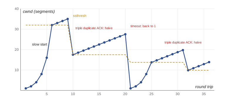
The resulting sawtooth gives a famous approximation, derived by Mathis and colleagues in 1997, for the average throughput of a long-lived Reno flow with maximum segment size MSS, round-trip time RTT and loss probability \(p\):
# Average throughput of a long TCP Reno flow: about 1.22 * MSS / (RTT * sqrt(p))
from math import sqrt
MSS = 1460 * 8
for rtt_ms, p in ((20, 1e-3), (100, 1e-3), (100, 1e-5), (100, 2e-10)):
    thr = 1.22 * MSS / (rtt_ms / 1000 * sqrt(p))
    print(f"RTT {rtt_ms:3d} ms, loss {p:7.0e}: {thr/1e6:10.1f} Mbit/s")
# loss rate needed for 10 Gbit/s at 100 ms
p_needed = (1.22 * MSS / (0.1 * 10e9)) ** 2
print(f"loss rate needed for 10 Gbit/s over 100 ms: {p_needed:.1e}")RTT 20 ms, loss 1e-03: 22.5 Mbit/s RTT 100 ms, loss 1e-03: 4.5 Mbit/s RTT 100 ms, loss 1e-05: 45.1 Mbit/s RTT 100 ms, loss 2e-10: 10076.0 Mbit/s loss rate needed for 10 Gbit/s over 100 ms: 2.0e-10
The last line explains why Reno struggles on modern long, fast paths: sustaining 10 Gbit/s over 100 ms requires a loss rate of about two in ten billion, far lower than real networks achieve, and after any loss Reno needs thousands of round trips of additive increase to regain its window. Note also that throughput is inversely proportional to RTT, so flows with long round trips get less than their share when competing with short ones.
Fairness
If \(K\) TCP flows share a bottleneck link of rate \(R\), we would like each to get about \(R/K\). Chiu and Jain showed in 1989 that additive increase with multiplicative decrease (AIMD) converges to such a fair share: when both flows increase additively, their difference stays the same, and when both halve, the difference halves. The simulation shows two flows starting far apart converging to equal shares. Fairness has limits in practice: applications can open many parallel connections to get more than one share, flows with shorter RTTs grow faster, and UDP applications that do not perform congestion control can take more than their share, which is why protocols over UDP such as QUIC and WebRTC implement their own congestion control.
# AIMD makes two flows converge to a fair share of a 100-unit link
x, y = 80.0, 10.0
for step in range(1, 61):
    if x + y > 100:            # loss: both halve
        x, y = x / 2, y / 2
    else:                      # no loss: both add 1
        x, y = x + 1, y + 1
    if step in (1, 10, 20, 40, 60):
print(f"step {step:2d}: flow A {x:5.1f} flow B {y:5.1f} difference {abs(x - y):5.1f}")step 1: flow A 81.0 flow B 11.0 difference 70.0 step 10: flow A 46.0 flow B 11.0 difference 35.0 step 20: flow A 56.0 flow B 21.0 difference 35.0 step 40: flow A 41.0 flow B 23.5 difference 17.5 step 60: flow A 30.5 flow B 21.8 difference 8.8
CUBIC and BBR
Most modern operating systems no longer use Reno. CUBIC, the default in Linux since 2006, in Windows and in macOS, and standardized in RFC 9438 in 2023, grows the window as a cubic function of the time since the last loss: quickly when far below the window at which the last loss occurred, slowly and cautiously near it, then quickly again to probe for newly available capacity. Because growth depends on elapsed time rather than on round trips, CUBIC is fairer between flows with different RTTs and fills long, fast paths much faster than Reno.
# CUBIC's window after a loss: W(t) = C (t - K)^3 + Wmax, independent of RTT
C, beta, Wmax = 0.4, 0.7, 100.0          # segments; beta is the window kept after a loss
K = ((Wmax * (1 - beta)) / C) ** (1 / 3)
print(f"K = {K:.2f} s to regain the previous maximum")
for t in (0, 1, 2, 3, K, 5, 6, 7):
    W = C * (t - K) ** 3 + Wmax
print(f"t = {t:4.1f} s W = {W:6.1f} segments")K = 4.22 s to regain the previous maximum t = 0.0 s W = 70.0 segments t = 1.0 s W = 86.7 segments t = 2.0 s W = 95.6 segments t = 3.0 s W = 99.3 segments t = 4.2 s W = 100.0 segments t = 5.0 s W = 100.2 segments t = 6.0 s W = 102.3 segments t = 7.0 s W = 108.6 segments
BBR, developed at Google and deployed for its services since 2016, takes a different approach. Instead of treating loss as the congestion signal, it builds a model of the path: it estimates the bottleneck bandwidth from the delivery rate and the minimum round-trip time, and paces packets at the estimated bandwidth while keeping about one bandwidth–delay product in flight. This avoids filling buffers, reduces queueing delay and keeps throughput high on paths with random loss, such as some wireless and long-haul links. Early versions could be unfair to loss-based flows such as CUBIC; BBRv2 and BBRv3 respond to loss and ECN as well. Delay-based and model-based congestion control remain an active research area, and QUIC implementations can choose their algorithm freely because they run in user space.
Worked problem
Time to reach full speed after a loss
A Reno flow on a path with a bandwidth–delay product of 10,000 segments and an RTT of 100 ms suffers a single loss at full window. How long does it take to regain the full window? How does CUBIC with C = 0.4 and beta = 0.7 compare?
Show solution
- Reno halves cwnd to 5,000 segments and adds one segment per RTT, so it needs 5,000 RTTs: 500 seconds, more than eight minutes.
- CUBIC keeps 70%, 7,000 segments, and regains \(W_{max}\) after \(K = \sqrt[3]{10000 \times 0.3 / 0.4} \approx 19.6\) seconds, regardless of the RTT.
- CUBIC recovers about 25 times faster on this path, which is why it replaced Reno as the default.
Answer: About 500 seconds for Reno versus about 20 seconds for CUBIC.
TCP and QUIC compared
QUIC, introduced in lesson 3, reimplements TCP's ideas over UDP with the benefit of hindsight. It combines the transport and TLS 1.3 handshakes into one round trip; multiplexes independent streams so that a loss blocks only one stream; uses packet numbers that are never reused, so acknowledgements are unambiguous and RTT estimates are always valid; acknowledges ranges of packets; supports connection migration through connection IDs; and encrypts nearly all of its header, preventing middleboxes from depending on, or interfering with, its details. Its loss detection and congestion control, described in RFC 9002, are close to TCP's, typically NewReno or CUBIC, with BBR also common. The trade-offs are higher processor cost and the occasional network that blocks UDP, in which case clients fall back to TCP.
| Feature | TCP | QUIC |
|---|---|---|
| Runs over | IP directly (protocol 6) | UDP |
| Where implemented | Operating system kernel | User-space library in the application |
| Handshake before data | 1 RTT, plus 1 RTT for TLS 1.3 | 1 RTT combined; 0-RTT when resuming |
| Streams | One byte stream per connection | Many independent streams |
| Head-of-line blocking across streams | Yes | No |
| Header visible to the network | Yes | Mostly encrypted |
| Connection identity | Four values: addresses and ports | Connection IDs, allowing migration |
Common mistakes
MistakeThinking TCP sequence numbers count segments.
InsteadThey count bytes: each sequence number is a byte position in the stream.
MistakeConfusing flow control with congestion control.
InsteadFlow control protects the receiver's buffer (rwnd); congestion control protects the network (cwnd).
MistakeBelieving slow start grows the window slowly.
InsteadSlow start doubles cwnd every RTT; it is slow only compared with sending a full window at once.
MistakeAssuming a timeout and a triple duplicate ACK are handled the same way.
InsteadReno halves cwnd after triple duplicate ACKs but drops to one segment after a timeout.
MistakeExpecting more bandwidth to fix low TCP throughput on a lossy long path.
InsteadLoss-based TCP throughput falls with RTT times the square root of loss; reduce loss, shorten the path or use a different algorithm.
MistakeThinking TIME_WAIT is a bug.
InsteadTIME_WAIT lets a lost final ACK be resent and lets old segments expire before addresses are reused.
Summary and key terms
- TCP provides a reliable, ordered, full-duplex byte stream with flow control and congestion control.
- Sequence and acknowledgement numbers count bytes; acknowledgements are cumulative, with SACK for selective recovery.
- The three-way handshake (SYN, SYN-ACK, ACK) costs one RTT; closing uses FIN in each direction and TIME_WAIT.
- Fast retransmit after three duplicate ACKs and an adaptive RTO based on SRTT and RTTVAR recover from loss.
- Flow control keeps unacknowledged data below the receiver's advertised window.
- Reno uses slow start, additive increase and multiplicative decrease; throughput is about 1.22 MSS/(RTT sqrt(p)).
- CUBIC grows the window as a cubic function of time; BBR models bandwidth and RTT; QUIC brings these ideas to user space over UDP.
- Three-way handshake
- The SYN, SYN-ACK and ACK exchange that opens a TCP connection.
- Cumulative acknowledgement
- An ACK number meaning all bytes before it have been received.
- Fast retransmit
- Retransmitting a segment after three duplicate ACKs, before the timer expires.
- Retransmission timeout (RTO)
- The time a sender waits for an ACK before retransmitting, computed from SRTT and RTTVAR.
- Receive window (rwnd)
- The free buffer space a receiver advertises for flow control.
- Congestion window (cwnd)
- A sender-side limit on unacknowledged data that adapts to network congestion.
- Slow start
- The phase in which cwnd doubles every RTT until it reaches ssthresh or a loss occurs.
- AIMD
- Additive increase, multiplicative decrease: the basis of TCP's fairness.
- CUBIC
- A congestion control algorithm whose window is a cubic function of time since the last loss.
- BBR
- A congestion control algorithm that paces sending using estimates of bottleneck bandwidth and minimum RTT.
Practice problems
Work each problem on paper first, then reveal the answer to check.
A segment carries bytes 1,000 to 1,499. What acknowledgement number confirms it, if all earlier bytes arrived?
Show answer
1,500.
Why are initial sequence numbers chosen randomly?
Show answer
To avoid confusion with old segments and make forged segments harder to inject.
What triggers fast retransmit?
Show answer
Three duplicate acknowledgements for the same byte.
With SRTT = 100 ms and RTTVAR = 10 ms, what is SRTT + 4 RTTVAR?
Show answer
140 ms (before applying any minimum RTO).
What does a receive window of zero mean?
Show answer
The receiver's buffer is full; the sender must stop and probe.
In slow start with no loss, how big is cwnd after 5 RTTs starting from 10 segments?
Show answer
320 segments.
What does Reno do after a timeout?
Show answer
Sets ssthresh to half of cwnd and restarts slow start from cwnd = 1.
Using the Mathis formula, how does throughput change if RTT doubles?
Show answer
It halves.
Why does AIMD converge to fairness?
Show answer
Additive increase keeps the difference between flows constant while multiplicative decrease halves it.
Name two ways QUIC improves on TCP for the web.
Show answer
A combined 1-RTT handshake, and independent streams without cross-stream head-of-line blocking.
Lesson quiz · 5 questions
Score 60% or more to complete this lesson.
Create a free account to save your progress, take quizzes and earn a certificate.