
CIV-450 · Lesson 4 of 12 · 19 min
Estimating for engineers
An engineer's estimate does several jobs at once. Early in a project it tells the owner whether the project is affordable and how much to budget. At tender it is the yardstick against which bids are judged, and the basis for deciding whether to award or retender. During construction it is the reference for pricing changes. Engineers who prepare estimates for owners do not need the full apparatus of a contractor's estimating department, which CON-200 and CON-300 cover in detail, but they do need to know how a contractor builds a price, where the uncertainty lies, and how to express that uncertainty honestly.
Estimate classes
Estimates are classified by the maturity of the design they are based on. The classification published by AACE International, widely used in North America, runs from Class 5, a concept screening estimate made with almost no design, to Class 1, a check estimate or bid made from complete documents. Each class has an expected accuracy range, wide and skewed upward for early estimates, narrowing as the design matures. The ranges are wider than many owners assume: a Class 5 estimate might be 50 % low or 100 % high. Early estimates are wrong more often by being too low than too high, because the unknown scope is mostly additional scope.
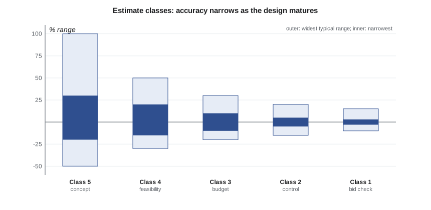
| Class | Design maturity | Typical method | Typical use |
|---|---|---|---|
| 5 | concept, 0 to 2 % | cost per lane-kilometre or similar unit | screening, long-range plans |
| 4 | feasibility, 1 to 15 % | parametric models, factored costs | options study, preliminary budget |
| 3 | preliminary design, 10 to 40 % | semi-detailed unit costs | budget authorization |
| 2 | detailed design, 30 to 75 % | detailed unit costs, takeoff | control estimate |
| 1 | complete, 65 to 100 % | detailed takeoff and pricing | engineer estimate, bid check |
Conceptual and parametric estimates
At the concept stage of the Ridgeway project, two years earlier, Kestrel Bay used historical costs from the city's recent road contracts: about CAD 3.5 million per kilometre for full urban reconstruction with storm sewers, plus separate allowances for the culvert, the wall and the roundabout. That Class 4 estimate, about CAD 7 million for construction, was enough to put the project in the capital plan. Parametric estimates of this kind work when the historical projects are similar and the costs are brought to the same date with a construction price index; they fail when the new project has unusual features, such as soft ground, which the historical average hides.
How a contractor builds a unit price
A contractor prices each item from its components. Direct costs are labour, equipment and materials, calculated from the crew, its production rate and the quantity. Subcontract prices are added for work the contractor does not self-perform. Then come indirect costs: the site office, supervision, temporary facilities, small tools, insurance and bonds, often called general conditions or site overhead. Finally the contractor adds home office overhead and profit. In a unit-price bid, all of these are spread over the unit prices, so a unit price for excavation includes a share of the superintendent's wages and the company's profit.
Worked problem
Building a unit price for excavation
A crew of one excavator with an operator and three trucks with drivers moves 900 m³ of clay a day. The crew costs CAD 9,450 a day including fuel and equipment. Site overhead and markup add 30 % to direct cost. What unit price per m³ results?
Show solution
- \[\text{direct} = 9450 / 900 = 10.50\ \text{per m}^3\]
- Disposal of surplus clay at a licensed site adds CAD 5.65 per m³ of material.
- \[\text{price} = (10.50 + 5.65) \times 1.30 = 21.00\ \text{per m}^3\]
Answer: The engineer's unit price of CAD 21.00 per m³ is consistent with this crew and haul.
Production rates drive the estimate. The same excavator moves far less soft wet clay than dry sand, and a crew that must stop for traffic every few minutes is slower than one working in a closed road. This is why the engineer's estimate should be built with the site in mind, not just from a price book: the varved clay, the two-stage traffic plan, the narrow working strip along the wall and the in-water work window all reduce production and raise costs.
The Ridgeway engineer's estimate
The Class 1 engineer's estimate for the tender follows the 16 items of the bid form. Quantities come from the takeoff of the final drawings, done by Sofia and checked by Owen. Unit prices come from recent city tenders, adjusted for date and site conditions, and from first-principles pricing of the items with no good history: the box culvert, the cofferdam and the retaining wall. A 5 % allowance covers mobilization, bonds and insurance, which the bid form carries as a separate lump sum.
# Engineer's estimate for the Ridgeway Road East and Kestrel Creek crossing contract,
# then a Monte Carlo range for the contingency
import random
UNITS = "SI"
SI = UNITS == "SI"
CUR = "CAD" if SI else "USD"
# item, unit, quantity, unit price  (unit prices include the contractor's overhead and profit)
if SI:
    items = [("Traffic control and staging", "LS", 1, 420000), ("Asphalt and curb removals", "m2", 9800, 9.0),
             ("Earth excavation", "m3", 14500, 21.0), ("Granular subbase", "m3", 4600, 55.0),
             ("Granular base", "m3", 2300, 72.0), ("Hot-mix asphalt, two lifts", "m2", 11500, 42.0),
             ("Concrete curb and gutter", "m", 3400, 85.0), ("Storm sewer, 300-900 mm", "m", 1150, 680.0),
             ("Catch basins and maintenance holes", "each", 46, 4800.0), ("Precast box culvert 4.5 x 2.4 m", "m", 26, 52000.0),
             ("Cofferdam and creek diversion", "LS", 1, 280000), ("Cantilever retaining wall", "m", 140, 5200.0),
             ("Roundabout at the operations centre", "LS", 1, 820000), ("Bioretention and low impact development", "LS", 1, 410000),
             ("Street lighting", "each", 48, 9800.0), ("Pavement markings and signs", "LS", 1, 110000)]
else:
    items = [("Traffic control and staging", "LS", 1, 330000), ("Asphalt and curb removals", "yd2", 11700, 7.0),
             ("Earth excavation", "yd3", 19000, 15.0), ("Granular subbase", "yd3", 6000, 38.0),
             ("Granular base", "yd3", 3000, 50.0), ("Hot-mix asphalt, two lifts", "yd2", 13750, 30.0),
             ("Concrete curb and gutter", "ft", 11150, 24.0), ("Storm sewer, 12-36 in.", "ft", 3770, 190.0),
             ("Catch basins and manholes", "each", 46, 3900.0), ("Precast box culvert 15 x 8 ft", "ft", 85, 12800.0),
             ("Cofferdam and creek diversion", "LS", 1, 220000), ("Cantilever retaining wall", "ft", 460, 1250.0),
             ("Roundabout at the operations center", "LS", 1, 640000), ("Bioretention and low impact development", "LS", 1, 320000),
             ("Street lighting", "each", 48, 7600.0), ("Pavement markings and signs", "LS", 1, 85000)]
sub = 0.0
for name, unit, q, p in items:
    sub += q * p
    print(f"{name:42s} {q:>8,} {unit:5s} x {p:>10,.2f} = {q*p:>12,.0f}")
mob = 0.05 * sub
print(f"{'Subtotal of unit-price items':42s} {sub:>40,.0f}")
print(f"{'Mobilization, bonds and insurance (5 %)':42s} {mob:>40,.0f}")
est = sub + mob
print(f"{'Engineer estimate (' + CUR + ')':42s} {est:>40,.0f}")
# uncertainty: triangular factors (low, most likely, high) on each item, plus a market factor on the whole bid
rng = {"Earth excavation": (0.90, 1.0, 1.35), "Precast box culvert": (0.95, 1.0, 1.30),
       "Cofferdam": (0.90, 1.0, 1.60), "Storm sewer": (0.92, 1.0, 1.20)}
random.seed(450)
runs = []
for _ in range(5000):
    tot = 0.0
    for name, unit, q, p in items:
        lo, ml, hi = next((v for k, v in rng.items() if name.startswith(k)), (0.93, 1.0, 1.10))
        tot += q * p * random.triangular(lo, hi, ml)
    tot *= 1.05 * random.triangular(0.94, 1.15, 1.0)
    runs.append(tot)
runs.sort()
pc = lambda f: runs[int(f * len(runs)) - 1]
print(f"\nMonte Carlo, 5,000 runs: P10 {pc(0.10):,.0f}  P50 {pc(0.50):,.0f}  P80 {pc(0.80):,.0f}  P90 {pc(0.90):,.0f}")
print(f"Chance the point estimate is not exceeded: {sum(r <= est for r in runs) / len(runs):.0%}")
print(f"Contingency to reach P80: {pc(0.80) - est:,.0f} ({(pc(0.80) - est) / est:.1%} of the estimate)")Traffic control and staging 1 LS x 420,000.00 = 420,000 Asphalt and curb removals 9,800 m2 x 9.00 = 88,200 Earth excavation 14,500 m3 x 21.00 = 304,500 Granular subbase 4,600 m3 x 55.00 = 253,000 Granular base 2,300 m3 x 72.00 = 165,600 Hot-mix asphalt, two lifts 11,500 m2 x 42.00 = 483,000 Concrete curb and gutter 3,400 m x 85.00 = 289,000 Storm sewer, 300-900 mm 1,150 m x 680.00 = 782,000 Catch basins and maintenance holes 46 each x 4,800.00 = 220,800 Precast box culvert 4.5 x 2.4 m 26 m x 52,000.00 = 1,352,000 Cofferdam and creek diversion 1 LS x 280,000.00 = 280,000 Cantilever retaining wall 140 m x 5,200.00 = 728,000 Roundabout at the operations centre 1 LS x 820,000.00 = 820,000 Bioretention and low impact development 1 LS x 410,000.00 = 410,000 Street lighting 48 each x 9,800.00 = 470,400 Pavement markings and signs 1 LS x 110,000.00 = 110,000 Subtotal of unit-price items 7,176,500 Mobilization, bonds and insurance (5 %) 358,825 Engineer estimate (CAD) 7,535,325 Monte Carlo, 5,000 runs: P10 7,576,061 P50 8,014,816 P80 8,388,262 P90 8,578,997 Chance the point estimate is not exceeded: 8% Contingency to reach P80: 852,937 (11.3% of the estimate)
The point estimate is CAD 7,535,325. The largest single item is the precast box culvert at CAD 1.35 million, followed by the roundabout, the storm sewer and the retaining wall. The culvert, the cofferdam, the wall and the excavation in soft clay together make up more than a third of the unit-price items, and that is where the uncertainty is concentrated.
Expressing uncertainty: the Monte Carlo range
A single number hides the most important information in an estimate, its uncertainty. Sofia's script assigns each item a triangular distribution: a low, most likely and high factor on its estimated cost. Most items get a narrow range of minus 7 % to plus 10 %. Excavation gets minus 10 % to plus 35 %, because the soft clay may need more subexcavation; the culvert minus 5 % to plus 30 %; the cofferdam minus 10 % to plus 60 %, because its cost depends on water levels during the work window; the storm sewer minus 8 % to plus 20 %. A market factor applied to the whole estimate, from minus 6 % to plus 15 %, represents the bidding climate. The simulation draws 5,000 combinations.
The results are striking. The point estimate of CAD 7.54 million has only about an 8 % chance of not being exceeded. The median is CAD 8.01 million, and the 80th percentile, P80, is CAD 8.39 million. The reason is that every distribution is skewed upward: the most likely value of each item is at the low end of its range, so adding the most likely values gives a total well below the likely total. The contingency needed to reach P80 is CAD 853,000, or 11.3 % of the estimate, which is the figure carried into the capital budget in lesson 1.
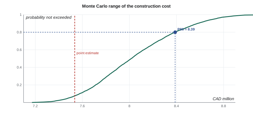
Two caveats keep this honest. First, the item ranges are judgements, and the analysis is only as good as the conversations that produced them; the team held a short risk workshop with Dr. Kowalczyk and the city's roads staff to set them. Second, the simulation treats items as independent, apart from the market factor. In reality, if the clay is worse than expected, excavation, the wall and the culvert will all cost more at once. Correlation widens the range, so the P80 above is, if anything, optimistic. More advanced practice models the main risks as events with probabilities and impacts, rather than as ranges on line items.
The estimate at tender
When bids arrive, the engineer's estimate is the benchmark. Bids within about 10 % of a good Class 1 estimate are normal. A low bid far below the estimate prompts a check of the low bidder's understanding of the scope and its unit prices; a cluster of bids well above it suggests either an error in the estimate or a risk that bidders priced and the estimator did not. In lesson 3, Northline's corrected bid of CAD 7.24 million came in 3.9 % below the estimate, and the spread of bids was about 9 %, a healthy result.
The engineer's estimate is usually kept confidential until bids close, because publishing it anchors bidders to it. Some agencies publish a budget range instead. Either way, the estimate and its basis, quantities, prices, sources and assumptions, should be documented well enough that someone else could check it, because it may be needed years later in a claim.
Practical points
- State the class and accuracy range with every estimate.
- Price items with no reliable history from crews, production rates and site conditions.
- Remember that most likely values do not add up to a likely total when ranges are skewed.
- Size contingency from a risk analysis, not a fixed percentage.
- Document the basis of the estimate for use in bid evaluation, changes and claims.
Common mistakes
MistakeQuoting an early estimate as a single figure without its range.
InsteadGive the class and the range; early estimates are uncertain and usually low.
MistakePricing from a price book without considering site conditions.
InsteadAdjust production rates for soft ground, traffic and working space.
MistakeAdding most likely values and calling the result the expected cost.
InsteadWith upward-skewed ranges, the sum of modes lies well below the median.
MistakeTreating every item as independent in a risk model.
InsteadCorrelated items, such as everything in soft clay, widen the range.
Summary and key terms
- Estimate classes run from Class 5 at concept to Class 1 at complete design, with narrowing accuracy ranges.
- Parametric estimates use historical unit costs adjusted for date and scope.
- A contractor's unit price includes direct costs, site overhead, home office overhead and profit.
- The Ridgeway engineer's estimate is CAD 7.54 million; the culvert is the largest item.
- A Monte Carlo simulation of skewed item ranges puts the point estimate at only about an 8 % chance of not being exceeded.
- Contingency of 11.3 % brings the budget to the 80th percentile.
- Engineer estimate
- The owner's independent estimate of the expected bid price, prepared from the final documents.
- Estimate class
- A category of estimate defined by design maturity, method and expected accuracy.
- Parametric estimate
- An estimate from historical costs per unit of a key parameter, such as length of road.
- Direct cost
- The cost of labour, equipment, materials and subcontracts for an item.
- Site overhead
- Project costs not tied to one item, such as supervision and site facilities.
- Production rate
- The quantity of work a crew completes per unit of time.
- Triangular distribution
- A probability distribution defined by low, most likely and high values.
- P80
- The value with an 80 % probability of not being exceeded.
Practice problems
Work each problem on paper first, then reveal the answer to check.
A crew costs CAD 6,200 a day and places 140 m of curb. With 35 % markup, what unit price results?
Show answer
6,200 / 140 × 1.35 = CAD 59.79 per metre.
Why is the sum of the most likely item costs usually below the median total?
Show answer
Each item's distribution is skewed upward, so its mean exceeds its mode; the means add, not the modes.
A Class 5 estimate is 10 million. What range might be reported?
Show answer
Roughly 5 to 20 million at the widest, using minus 50 % to plus 100 %.
How would correlation between the excavation, wall and culvert costs change the P80?
Show answer
It would widen the distribution and raise the P80.
Lesson quiz · 5 questions
Score 60% or more to complete this lesson.
Create a free account to save your progress, take quizzes and earn a certificate.