Filtration and membranes

Settled water still carries fine flocs, some clay and a share of the pathogens that entered with the river. Filtration is the final particle barrier, and in a conventional plant it is the step that earns most of the regulatory credit for removing Giardia and Cryptosporidium. Its performance is judged continuously by filtered water turbidity, which is why the 0.3 NTU rule of lesson 1 applies to every filter. This lesson covers granular media filtration, which the new plant will use, and the membrane alternative that Willowbend compared with it.

How a granular filter works

A rapid granular filter is a bed of sand, or sand under a layer of coarser anthracite coal, about 0.6 to 1.2 m deep, through which water flows downward at 5 to 15 m/h (about 2 to 6 gpm/ft²). The pores between grains are tens to hundreds of micrometres across, far larger than most particles removed, so straining is not the main mechanism. Instead, particles are transported to grain surfaces by gravity settling, by interception as streamlines pass close to a grain, and, for the smallest particles, by Brownian diffusion; then they attach if they have been destabilized by coagulation. This is why a filter cannot be operated without proper coagulation upstream: unconditioned particles reach the grains but do not stick, and they pass straight through.

Capture is a depth process, so the bed gradually fills with deposits from the top down. Two things end a filter run: the head loss through the clogging bed reaches the available head, typically 2 to 3 m, or particles begin to break through and the filtered turbidity rises. A well-designed filter reaches terminal head loss slightly before breakthrough, so that it is backwashed while still producing good water. Typical runs last 24 to 72 hours.

Filter media

Media are described by the effective size, the sieve opening that passes 10 % of the grains by mass (\(d_{10}\)), and the uniformity coefficient, the ratio \(d_{60}/d_{10}\). Typical rapid filter sand has an effective size of 0.45 to 0.55 mm and a uniformity coefficient below 1.5; anthracite has an effective size of 0.9 to 1.1 mm. In a dual-media filter, the lighter and coarser anthracite sits on top after backwashing and the heavier, finer sand underneath, so the water meets coarse pores first and fine pores later. Deposits spread through a greater depth, giving longer runs at higher rates. Some plants replace the anthracite with granular activated carbon, which adds adsorption of taste and odour compounds and organic matter, as lesson 7 discusses.

Head loss through a clean bed

The head loss through a clean bed of media is found from the Carman-Kozeny or Ergun equations, which treat the bed as a bundle of tortuous channels. In the Ergun form,

where \(L\) is the bed depth, \(d\) the grain diameter, \(\phi\) the sphericity of the grains (about 0.8 for sand, 0.7 for angular anthracite), \(\varepsilon\) the porosity (0.40 to 0.45 for sand, 0.47 to 0.52 for anthracite), and \(v\) the filtration rate as a superficial velocity. At filtration rates the flow is laminar and the first term dominates, so head loss is nearly proportional to velocity and to viscosity, and is highest in cold water.

# Clean-bed head loss (Carman-Kozeny), filter count and a membrane comparison
UNITS = "SI"
SI = UNITS == "SI"
g, rho, mu = 9.81, 1000.0, 1.52e-3            # water at 5 C
def hl_ck(v, L, d, eps, phi):                  # clean-bed head loss, m (v in m/s, L and d in m)
    Re = phi * rho * v * d / mu
    f = 150 * (1 - eps) / Re + 1.75
    return f * (L / (phi * d)) * ((1 - eps) / eps**3) * v**2 / g, Re
Qp = 60000.0 if SI else 16.0 * 3785.4          # m3/d peak
rate = 10.0                                    # m/h design filtration rate (about 4 gpm/ft2)
layers = [("anthracite", 0.60, 1.0e-3, 0.50, 0.73), ("sand", 0.30, 0.5e-3, 0.42, 0.82)]
v = rate / 3600
tot = 0
for name, L, d, eps, phi in layers:
    h, Re = hl_ck(v, L, d, eps, phi)
    tot += h
    print(f"{name:10s} L = {L:.2f} m  d = {d*1000:.1f} mm  Re = {Re:.2f}  clean-bed head loss {h:.3f} m" if SI else
          f"{name:10s} L = {L*39.37:.0f} in.  d = {d*1000:.1f} mm  Re = {Re:.2f}  clean-bed head loss {h*3.281:.2f} ft")
print(f"total clean-bed head loss {tot:.2f} m" if SI else f"total clean-bed head loss {tot*3.281:.2f} ft")
area = Qp / 24 / rate
for n in (6, 8, 10):
    a1 = area / (n - 1)                        # one filter out of service for backwash
    print(f"{n} filters, one out of service: {a1:.0f} m2 each" if SI else
          f"{n} filters, one out of service: {a1*10.764:,.0f} ft2 each")
# membranes instead: ultrafiltration at a design flux of 50 L/(m2 h) after recovery losses
flux = 50.0
recovery = 0.95
feed = Qp / recovery
Amem = feed * 1000 / 24 / flux
print(f"UF option: feed {feed:,.0f} m3/d, membrane area {Amem:,.0f} m2, about {Amem/55:,.0f} modules of 55 m2" if SI else
      f"UF option: feed {feed/3785.4:.1f} MGD, membrane area {Amem*10.764:,.0f} ft2 at {flux/1.698:.0f} gfd, about {Amem/55:,.0f} modules of 590 ft2")

anthracite L = 0.60 m  d = 1.0 mm  Re = 1.33  clean-bed head loss 0.150 m
sand       L = 0.30 m  d = 0.5 mm  Re = 0.75  clean-bed head loss 0.531 m
total clean-bed head loss 0.68 m
6 filters, one out of service: 50 m2 each
8 filters, one out of service: 36 m2 each
10 filters, one out of service: 28 m2 each
UF option: feed 63,158 m3/d, membrane area 52,632 m2, about 957 modules of 55 m2

At 10 m/h and 5 °C, the clean dual-media bed loses about 0.15 m through 0.6 m of anthracite and 0.53 m through 0.3 m of sand, about 0.7 m in all before any deposits accumulate. With 2.4 m of head available above the media, the remaining 1.7 m is the head the bed can use for clogging before it must be backwashed.

Sizing the filters

At the peak flow of 60,000 m³/d and a design rate of 10 m/h, the plant needs 250 m² of filter area in service. With the largest filter out for backwashing or repair, eight filters of about 36 m² each, built as 4.5 m by 8 m cells, provide the area. The team chooses eight filters rather than six because smaller cells backwash with less water and a smaller backwash pump, and the loss of one filter shifts less load onto the others.

Each filter has its own effluent turbidity meter, as most regulators require, and a rate-of-flow controller. The design uses constant-rate control, in which a valve opens gradually as the bed clogs so that each filter delivers its share of the flow. The alternative, declining-rate filtration, lets each filter's rate fall as it clogs and is simpler but makes the effluent quality more variable.

Backwashing

A clogged filter is cleaned by reversing the flow. Clean water is pumped up through the underdrain at a rate high enough to expand the bed by 20 to 40 %, so that grains rub against one another and release their deposits, which are carried over troughs to waste. Typical backwash rates are 35 to 60 m/h (15 to 25 gpm/ft²) for 8 to 15 minutes, preceded by air scour at 50 to 90 m/h of air to break up deposits. The backwash rate must be high enough to fluidize the coarsest media but not so high that it carries anthracite over the troughs; because water viscosity changes, the rate is adjusted with temperature.

After backwashing, a filter typically produces water of higher turbidity for 15 to 60 minutes while the bed ripens. Filter-to-waste, which sends this first filtrate to waste, protects the clearwell from the turbidity spike and the pathogens that can accompany it. Spent backwash water amounts to 2 to 4 % of production; it is usually settled and the clarified water recycled to the plant inlet, a practice that US rules require to be returned ahead of the point of primary coagulant addition.

Monitoring filter performance

Each filter's effluent turbidity is recorded continuously, and the combined filter effluent is the compliance point. Many plants also install particle counters, which count particles in size ranges such as 2 to 5 µm, the size of Cryptosporidium oocysts, and can show a filter starting to deteriorate before turbidity rises. Operators watch three moments in every run: the ripening period after backwash, the steady middle of the run, and the approach to terminal head loss, when breakthrough is most likely. A sudden change in flow, such as starting a filter at full rate or switching another filter to backwash, can dislodge deposits and cause a spike; slow-start valves and gradual rate changes avoid it. Filter media are inspected and cored periodically to check for mud balls, cracking and loss of media, which signal inadequate backwashing.

Slow sand and biological filtration

Slow sand filters operate at only 0.1 to 0.4 m/h without coagulation. A biologically active layer, the schmutzdecke, forms on the sand surface and removes particles, pathogens and some organic matter. They are simple and very effective for small communities with clean source water but need large areas and are clogged quickly by turbid prairie rivers. Rapid filters can also be operated biologically: when no chlorine is applied ahead of them, bacteria colonize the media and consume biodegradable organic carbon, reducing regrowth in the distribution system. Biological filtration is often combined with ozone, which breaks large organic molecules into biodegradable fragments.

Membrane filtration

Membranes separate particles by size at a barrier with defined pores. Microfiltration (MF) membranes have pores of about 0.1 µm and ultrafiltration (UF) about 0.01 µm; both remove essentially all protozoa and bacteria and much of the virus load, and they receive regulatory credit of 4-log or more for Giardia and Cryptosporidium where integrity is verified. Nanofiltration (NF) removes hardness, colour and much organic carbon, and reverse osmosis (RO) removes nearly all dissolved salts.

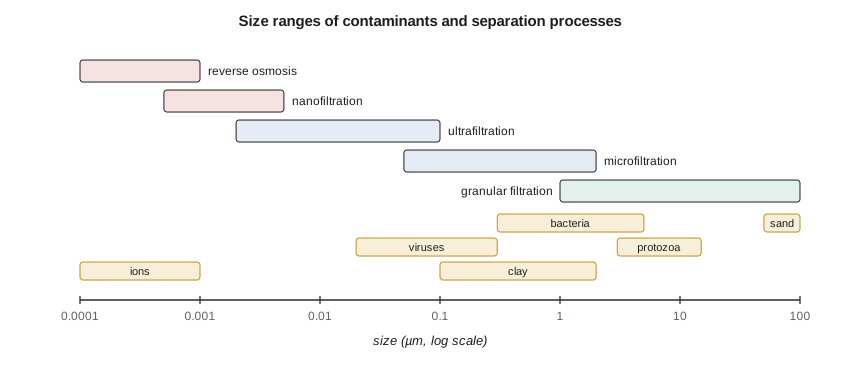
Low-pressure MF and UF systems run at transmembrane pressures of 30 to 150 kPa (5 to 20 psi) and fluxes of 40 to 100 L/(m²·h), or about 25 to 60 gal/(ft²·d). Hollow fibres are assembled into modules of tens of square metres. Fouling by particles, organic matter and biofilm gradually raises the pressure needed; it is controlled by backwashing every 20 to 60 minutes and by chemical cleaning every few weeks or months. Integrity is checked daily by a pressure decay test, in which the feed side is pressurized with air and the rate of pressure loss shows whether any fibre is broken.

Membranes receive higher pathogen credit than granular filters and produce consistently low turbidity, but they do not remove dissolved organic carbon unless coagulant is added ahead of them, and they produce a waste stream of 5 to 10 % of the feed. The comparison in the script shows that a UF plant would need over 50,000 m² of membrane, close to 1,000 modules, with their periodic replacement every 7 to 10 years.

Willowbend's life-cycle comparison, prepared with the city's operators, finds the two options within 10 % of each other in present cost. The city chooses dual-media filtration, because it already has staff experienced with conventional plants and because coagulation is needed for organic removal in either case, but asks that the filter building be laid out so that membranes could replace the filters at their first major refurbishment.