Short columns: axial load and bending

Columns carry the floors above them down to the foundations. Almost every column carries some bending as well as axial load, from unbalanced floor spans, frame action under wind, or simply the unavoidable eccentricity of construction. This lesson develops the strength of a short column, one in which the extra moment from lateral deflection is negligible, under combined axial load and bending. The tool for this is the interaction diagram, built by the same strain-compatibility method used for beams in lesson 4. The example is the ground-floor interior column of the office building.

Types of columns

Most concrete columns are tied columns: longitudinal bars held in position by rectangular ties at regular spacing. Spiral columns have their bars arranged in a circle and enclosed by a continuous helix of closely spaced wire or bar. The spiral confines the core concrete so well that after the cover spalls off the column can carry its load at large deformations, which is why spiral columns get a higher resistance factor and a higher maximum axial load. Composite columns encase a structural steel shape in concrete or fill a steel tube with concrete.

Columns are also classed by slenderness. A short column fails by material failure, crushing of the concrete or yielding of the steel, at the load given by its cross-section. A slender column deflects laterally under load, the axial load acting on that deflection adds moment, and the column fails at a lower load. Most building columns braced against sway are short; lesson 11 covers slender ones.

Axial load capacity

Under concentric axial load, the concrete and steel shorten together. The concrete reaches its capacity at a strain of about 0.002, at which point Grade 400 or Grade 60 steel has just yielded, so the strength is the sum of the two contributions:

The factor \(\alpha_1\) reflects the lower strength of concrete in a column compared with a cylinder, caused by the size, the casting position and the sustained nature of the load. No real column is perfectly concentric, so A23.3 caps the factored axial resistance at \(P_{r,max} = 0.80P_{ro}\) for tied columns and \(0.85P_{ro}\) for spiral columns. That cap allows for an accidental eccentricity of roughly 10 per cent of the column depth.

The steel ratio \(\rho_g = A_{st}/A_g\) must be between 1 and 8 per cent. The lower limit gives some resistance to bending and controls creep, which slowly shifts load from the concrete to the steel. The upper limit avoids congestion; in practice 4 per cent is a sensible maximum where bars are lap-spliced, because the laps double the steel at the splice. Rectangular tied columns need at least four bars, one in each corner.

Axial load with bending

When a column carries a moment \(M\) together with an axial load \(P\), the load acts as if it were applied at an eccentricity \(e = M/P\) from the centroid. A small eccentricity puts the whole section in compression and the column fails by crushing. A large eccentricity puts the far face in tension, the far steel yields, and the column behaves more like a beam. Between these lies the balanced condition, in which the concrete reaches its crushing strain at the same moment that the extreme tension steel reaches its yield strain.

For each assumed position of the neutral axis there is one strain profile, one set of bar stresses and one pair of resultants \((P, M)\). Sweeping the neutral axis from far outside the section (pure compression) to near the compression face (tension) traces out a curve: the interaction diagram. Any combination of factored load and moment that falls inside the curve is safe.

Here \(C_c = \alpha_1\phi_c f'_c ab\), \(y_i\) is the depth of bar layer \(i\) from the compression face, \(f_{si} = E_s\varepsilon_{si}\) limited to \(\pm f_y\) and taken positive in compression, and the concrete displaced by compression bars inside the stress block is subtracted. Because the material factors are inside every term, each point is already a factored resistance; A23.3 needs no further reduction.

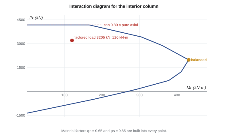
The diagram has a recognizable shape. From the capped top, increasing moment lowers the axial capacity in the compression-controlled region. At the balanced point the moment capacity is a maximum (for the factored diagram of a symmetrical section). Below balanced, in the tension-controlled region, a little axial compression actually increases the moment capacity, because it delays yielding of the tension steel. This last fact matters: a column with low axial load and high moment is unconservative to check with the largest axial load, so designers check the combinations with minimum axial load too, such as 0.9D with wind.

The office column

The ground-floor interior column supports two floors and the roof over a 7.5 m × 7.5 m tributary area. From the floor and roof loads and the column self-weight, Owen finds specified loads of \(D = 1700\) kN and \(L = 720\) kN (with the live load reduction the building code allows for large tributary areas). The frame analysis of CIV-321 gives a factored moment of 120 kN·m from unbalanced live load on the adjacent spans. The factored axial load is \(P_f = 1.25(1700) + 1.5(720) = 3205\) kN. Priya has proposed 500 × 500 mm columns with 8-25M bars (three per face), \(f'_c = 30\) MPa.

Computing a full diagram by hand is tedious, so Sofia extends the strain-compatibility routine of lesson 4 to a net axial force and sweeps the neutral axis depth. She also interpolates the moment capacity at the factored axial load.

# Interaction diagram for a tied column, CSA A23.3 (factored resistances)
fc, fy, Es, ecu = 30.0, 400.0, 200000.0, 0.0035
phic, phis = 0.65, 0.85
b = h = 500.0
layers = [(3 * 500.0, 64.0), (2 * 500.0, 250.0), (3 * 500.0, 436.0)]   # 8-25M
a1 = max(0.85 - 0.0015 * fc, 0.67); b1 = max(0.97 - 0.0025 * fc, 0.67)
Ag = b * h; Ast = sum(A for A, _ in layers)
Pro = a1 * phic * fc * (Ag - Ast) + phis * fy * Ast
Prmax = 0.80 * Pro

def point(c):
    a = min(b1 * c, h)
    Cc = a1 * phic * fc * a * b
    P = Cc; M = Cc * (h / 2 - a / 2)
    for As, y in layers:
        es = ecu * (c - y) / c
        fs = max(-fy, min(fy, Es * es))
        f = phis * As * fs - (a1 * phic * fc * As if y < a else 0)
        P += f; M += f * (h / 2 - y)
    return P / 1e3, M / 1e6

print(f"rho = {Ast/Ag*100:.2f}%, Pro = {Pro/1e3:.0f} kN, Pr,max = {Prmax/1e3:.0f} kN")
cb = ecu / (ecu + fy / Es) * 436
print("    c (mm)    Pr (kN)   Mr (kN.m)")
pts = []
for c in (600, 500, 400, 350, cb, 200, 150, 100, 60):
    P, M = point(c)
    pts.append((P, M))
    tag = "  balanced" if c == cb else ""
    print(f"{c:9.0f} {min(P, Prmax/1e3):10.0f} {M:10.0f}{tag}")
# pure bending: find c with P = 0 by bisection
lo, hi = 1.0, 250.0
for _ in range(60):
    c = (lo + hi) / 2
    lo, hi = (lo, c) if point(c)[0] > 0 else (c, hi)
print(f"pure bending: c = {c:.0f} mm, Mr = {point(c)[1]:.0f} kN.m")
# check the ground-floor interior column: Pf = 3205 kN, Mf = 120 kN.m
Pf, Mf = 3205, 120
pts.sort()
for (P1, M1), (P2, M2) in zip(pts, pts[1:]):
    if P1 <= Pf <= P2:
        Mcap = M1 + (M2 - M1) * (Pf - P1) / (P2 - P1)
print(f"at Pf = {Pf} kN the diagram gives Mr = {Mcap:.0f} kN.m vs Mf = {Mf} -> {'OK' if Mf <= Mcap and Pf <= Prmax/1e3 else 'not OK'}")

rho = 1.60%, Pro = 5222 kN, Pr,max = 4177 kN
    c (mm)    Pr (kN)   Mr (kN.m)
      600       4177         49
      500       4177        166
      400       3423        305
      350       2880        361
      277       1984        431  balanced
      200       1233        411
      150        690        378
      100        150        294
       60       -488        178
pure bending: c = 89 mm, Mr = 268 kN.m
at Pf = 3205 kN the diagram gives Mr = 327 kN.m vs Mf = 120 -> OK

At \(P_f = 3205\) kN the column resists 327 kN·m against a demand of 120 kN·m, so the section is controlled by axial load rather than moment. Priya considers reducing the bars to 8-20M, but keeps 8-25M because the same column size continues to the roof, where moments from the roof frame are larger relative to the axial load, and because a uniform bar size simplifies splices.

The table of points also shows why the interaction diagram matters even for a lightly loaded column. Near pure bending the capacity is lowest; adding axial load up to the balanced point increases it. If the roof column carries only a small axial load with a large wind moment, its capacity comes from the lower part of the curve, and that is where it may govern.

Biaxial bending

Corner columns and columns in two-way frames carry moments about both axes. The exact solution needs a three-dimensional interaction surface. A simple, widely used approximation is the Bresler reciprocal load equation, which estimates the capacity under biaxial bending from the uniaxial capacities:

where \(P_{rx}\) and \(P_{ry}\) (or \(P_{nx}\), \(P_{ny}\)) are the axial capacities at the actual eccentricity about each axis alone. The equation is accurate when axial load is significant, above about a tenth of the pure axial capacity. For lower loads, the section is checked as a beam in biaxial bending, or a computer program integrates the stresses over the section for an inclined neutral axis.

Practical column design

• Size columns for axial load first: with 1.5 to 2 per cent steel, a tied column resists a factored axial load of roughly \(0.5f'_c A_g\) at its cap, so \(A_g \approx 2P/f'_c\) is a good first guess; then check moments with the interaction diagram.
• Keep column sizes constant over several floors and vary the steel and concrete strength, so formwork can be reused. Higher-strength concrete in lower storeys is common.
• Columns from 300 mm (12 in.) upward are common; very small columns are hard to cast and congested at beam-column joints.
• Symmetrical reinforcement is used because moments usually reverse under wind and pattern loads.
• Load combinations with minimum axial load must be checked, because they may govern in the tension-controlled region.