
CHE-460 · Lesson 7 of 12 · 21 min
Recycle, tear streams and convergence
Once the rigorous reactor and columns were in, the ester line model began to take longer to converge, and on some cases it stopped converging at all. Theo had two recycles in the flowsheet: the ester column distillate returning to the decanter, and the recovered acid and ethanol returning to the mixer. Both had been converged by the simulator's default method with default settings. When he added the n-propanol that arrives as a trace in the fresh ethanol, the recycle loop took hundreds of iterations, and on one case gave up. Ingrid tells him to stop clicking run and find out what the solver is doing.
Why recycles need iteration
In a sequential-modular simulator, each unit is calculated from its inlet streams. A recycle stream is an inlet to an early unit and an outlet of a later one. When the calculation starts, it is not known. The simulator chooses a tear stream, guesses its values, calculates round the loop, and compares the calculated tear with the guess. If they differ by more than a tolerance, it updates the guess and goes round again. The whole loop can be written as a function that maps a guess \(x\) to a calculated value \(g(x)\); the converged solution is a fixed point where \(x = g(x)\).
The choice of tear stream matters. A good tear stream breaks every recycle loop in the flowsheet with as few streams, or as few variables, as possible. Simulators choose tears automatically by analysing the flowsheet's structure, but the user can override them, and should when the automatic choice is poor. A tear stream with a well-known value, such as a recycle whose flow is set by the design basis, is a good choice, because the first guess is close. In Theo's flowsheet, the two tears are stream S9, the distillate, and stream S12, the acid and ethanol recycle.
Direct substitution
Direct substitution simply takes the calculated value as the next guess. It is safe, in that it seldom diverges for physical recycles, and slow, because its rate of convergence depends on how strongly the recycle feeds back on itself. For a single variable, the error shrinks each iteration by a factor equal to the slope of \(g\) near the solution. A recycle that returns a large fraction of a component, so that the slope is close to one, converges very slowly. Trace components that are recycled almost completely, with only a small exit, are the classic case: they build up over hundreds of passes.
That is exactly the n-propanol problem. The fresh ethanol carries 0.20 kmol/h of propanol. Propanol is barely reactive in the loop, and the separations return almost all of it to the mixer. The only way out is the small fraction that leaves in the products and waste water. In steady state the propanol in the recycle must build up until the exit rate equals the entry rate, at 6.47 kmol/h, more than thirty times the fresh rate. Direct substitution approaches that value by a small step each pass.
# Converging a recycle loop: direct (successive) substitution versus Wegstein acceleration, and the effect of a purge
import math
fresh = {"acid": 26.4, "ethanol": 26.3, "propanol": 0.20}   # kmol/h; propanol is a trace impurity in the ethanol
def Xeq(M, K=4.0):
    a, b, c = 1 - 1 / K, -(1 + M), M
    return (-b - math.sqrt(b * b - 4 * a * c)) / (2 * a)
def loop(r, purge):
    """One pass round the loop: guess recycle r (acid, ethanol, propanol) -> calculated recycle."""
    acid = fresh["acid"] + r[0]; eth = fresh["ethanol"] + r[1]; pr = fresh["propanol"] + r[2]
    X = 0.90 * Xeq(eth / acid)                     # pre-reactor reaches 90 % of equilibrium
    ra = X * acid
    acid_out, eth_out = acid - ra, eth - ra
    # separation train returns most unreacted material; propanol follows the ethanol
    back = [0.96 * acid_out, 0.97 * eth_out, 0.97 * pr]
    return [b * (1 - purge) for b in back], X
def solve(method, purge, tol=1e-6, maxit=1000, qmin=-5.0):
    x = [0.0, 0.0, 0.0]; hist = []
    gx, _ = loop(x, purge); x_old, g_old = x, gx
    x = gx
    for it in range(1, maxit + 1):
        gx, X = loop(x, purge)
        err = max(abs(a - b) for a, b in zip(gx, x)); hist.append(err)
        if err < tol: return x, X, it, hist
        if method == "direct":
            xn = gx
        else:   # Wegstein, applied to each tear variable, with q bounded to keep it stable
            xn = []
            for i in range(3):
                dx = x[i] - x_old[i]
                s = (gx[i] - g_old[i]) / dx if abs(dx) > 1e-12 else 0.0
                q = s / (s - 1) if abs(s - 1) > 1e-12 else 0.0
                q = max(qmin, min(0.0, q))
                xn.append(q * x[i] + (1 - q) * gx[i])
        x_old, g_old, x = x, gx, xn
    return x, X, maxit, hist
for method, qmin in (("direct", 0), ("wegstein", -5.0), ("wegstein", -50.0)):
    r, X, it, hist = solve(method, purge=0.0, qmin=qmin)
    label = method if method == "direct" else f"{method} q >= {qmin:g}"
    print(f"{label:18s}: {it:3d} iterations; recycle acid {r[0]:.2f}, ethanol {r[1]:.2f}, propanol {r[2]:.2f} kmol/h; X = {X:.3f}")
    print("                    error after iterations 1, 5, 10, 20: " + ", ".join(f"{hist[i]:.1e}" for i in (0, 4, 9, 19) if i < len(hist)))
# Newton's method on the residual F(r) = g(r) - r with a finite-difference Jacobian
def gauss(A, b):
    n = len(b); M = [row[:] + [bb] for row, bb in zip(A, b)]
    for c in range(n):
        p = max(range(c, n), key=lambda r_: abs(M[r_][c])); M[c], M[p] = M[p], M[c]
        for r_ in range(c + 1, n):
            f = M[r_][c] / M[c][c]
            M[r_] = [a - f * bq for a, bq in zip(M[r_], M[c])]
    x = [0.0] * n
    for r_ in range(n - 1, -1, -1):
        x[r_] = (M[r_][n] - sum(M[r_][k] * x[k] for k in range(r_ + 1, n))) / M[r_][r_]
    return x
r = [0.0, 0.0, 0.0]
for it in range(1, 20):
    g0, X = loop(r, 0.0); F0 = [a - b for a, b in zip(g0, r)]
    if max(map(abs, F0)) < 1e-6: break
    J = [ [0.0] * 3 for _ in range(3)]
    for j in range(3):
        rp = r[:]; h = 1e-6 * max(1.0, abs(r[j])); rp[j] += h
        gp, _ = loop(rp, 0.0)
        for i in range(3): J[i][j] = ((gp[i] - rp[i]) - F0[i]) / h
    d = gauss(J, [-f for f in F0]); r = [a + b for a, b in zip(r, d)]
print(f"newton            : {it - 1:3d} iterations; recycle acid {r[0]:.2f}, ethanol {r[1]:.2f}, propanol {r[2]:.2f} kmol/h (3 extra loop passes each for the Jacobian)")
print()
print("purge fraction   propanol in recycle   ethanol lost in purge")
for p in (0.0, 0.005, 0.01, 0.02, 0.05):
    r, X, it, _ = solve("wegstein", purge=p, qmin=-50.0)
    back = r[1] / (1 - p)
print(f" {p:5.3f} {r[2]:6.2f} kmol/h {back * p:6.2f} kmol/h")direct : 400 iterations; recycle acid 15.53, ethanol 17.69, propanol 6.47 kmol/h; X = 0.614
error after iterations 1, 5, 10, 20: 4.0e+00, 1.7e-01, 1.4e-01, 1.1e-01
wegstein q >= -5 : 164 iterations; recycle acid 15.53, ethanol 17.69, propanol 6.47 kmol/h; X = 0.614
error after iterations 1, 5, 10, 20: 4.0e+00, 8.5e-02, 3.2e-02, 8.6e-03
wegstein q >= -50 : 76 iterations; recycle acid 15.53, ethanol 17.69, propanol 6.47 kmol/h; X = 0.614
error after iterations 1, 5, 10, 20: 4.0e+00, 1.9e-01, 4.9e-03, 1.4e-03
newton : 2 iterations; recycle acid 15.53, ethanol 17.69, propanol 6.47 kmol/h (3 extra loop passes each for the Jacobian)
purge fraction propanol in recycle ethanol lost in purge
0.000 6.47 kmol/h 0.00 kmol/h
0.005 5.54 kmol/h 0.09 kmol/h
0.010 4.84 kmol/h 0.17 kmol/h
0.020 3.85 kmol/h 0.34 kmol/h
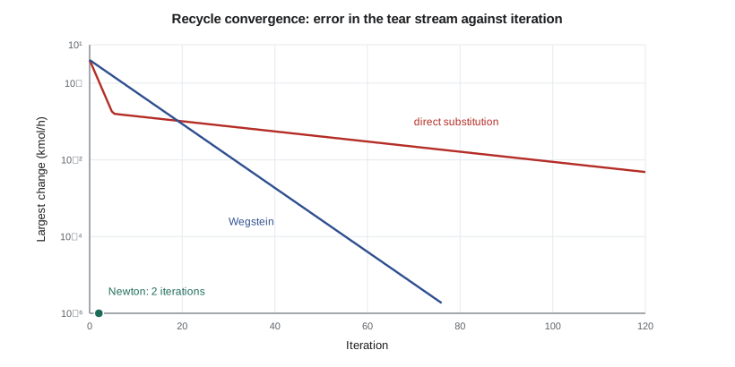
0.050 2.35 kmol/h 0.82 kmol/hDirect substitution had not converged to the tolerance after 400 iterations; the error after 20 was still 0.11 kmol/h. Its final values happen to be right, but only because the loop's slow components were nearly settled when it stopped.
Wegstein acceleration
The Wegstein method, published by J. H. Wegstein in 1958 and the default in many sequential-modular simulators, speeds up direct substitution by estimating the slope of \(g\) from the last two iterations and extrapolating towards the fixed point. It is applied to each tear variable separately.
When \(q = 0\) this is direct substitution. Negative values of \(q\) accelerate; positive values damp. Because the slope estimate can be poor, simulators bound \(q\), commonly between about −5 and 0. The code shows the effect. With \(q\) bounded at −5, Wegstein converged in 164 iterations instead of over 400. For the propanol, whose slope is very close to one, the ideal \(q\) is far below −5, and relaxing the bound to −50 cut the count to 76. Relaxing bounds is not free: in a loop with interacting variables, aggressive acceleration can overshoot and oscillate. Theo relaxes the bound only on the propanol variable.
Newton and quasi-Newton methods
Newton's method treats the recycle as a set of equations \(F(x) = g(x) - x = 0\) and solves them using the Jacobian matrix of partial derivatives. Each Newton step needs the Jacobian, which a sequential-modular simulator must estimate by perturbing each tear variable in turn and recalculating the loop. For three tear variables, that is three extra loop passes per iteration. In return, Newton converges quadratically near the solution. In the code it converged in two iterations, or eight loop passes in total. Quasi-Newton methods such as Broyden's update the Jacobian from the iterations already done, avoiding most of the perturbation passes. They are the usual choice for loops with many interacting tear variables, and for convergence of design specifications together with tears.
| Method | Information used | Speed | Robustness |
|---|---|---|---|
| Direct substitution | Last calculated value | Slow for strong recycles | High for physical loops |
| Wegstein | Slope of each variable from two iterations | Fast for weakly interacting variables | Good with bounds |
| Broyden (quasi-Newton) | Approximate Jacobian updated each pass | Fast; superlinear | Moderate; needs a fair start |
| Newton | Full Jacobian by perturbation | Quadratic near solution | Needs a good start |
Worked problem
Wegstein by hand
For a single tear variable, \(x_{1} = 5.0\) gives \(g(x_{1}) = 5.5\) and \(x_{2} = 5.5\) gives \(g(x_{2}) = 5.95\). Find the Wegstein update.
Show solution
- Slope \(s = (5.95 - 5.5) / (5.5 - 5.0) = 0.9\).
- \(q = 0.9 / (0.9 - 1) = -9\). If bounded at −5, use \(q = -5\).
- Unbounded: \(x_{3} = -9 \times 5.5 + 10 \times 5.95 = 10.0\).
- Check: with a linear \(g\) of slope 0.9 through these points, the fixed point is \(5.95 + 0.9(x - 5.5) = x\), giving \(x = 10.0\).
Answer: The unbounded update jumps straight to 10.0, the exact fixed point for a linear loop. With the bound of −5 it would reach 8.2 and need more passes.
Purges and the meaning of a slow recycle
A slow recycle is often telling the engineer something about the plant, not only about the solver. Propanol accumulates because the plant has almost no exit for it. In the real plant it would build up over days, raising the propanol in the ester product and eventually affecting quality. The cure is a purge: a small bleed from the recycle that removes accumulating components, at the cost of some ethanol and acid lost with it. The second part of the code shows the trade-off. A purge of 1 % of the recycle cuts the propanol held in the loop from 6.47 to 4.84 kmol/h, and loses 0.17 kmol/h of ethanol. Lesson 9 finds the best purge fraction by optimization.
Convergence tolerances deserve care too. A loose tolerance on the tear stream leaves an error that shows up as a mass balance that does not quite close. A tight tolerance on a stream with large flows may be unattainable in floating-point arithmetic, and on trace components may be meaningless. Simulators use relative tolerances on each variable, often with a floor for small flows. Theo sets the tolerance at 0.01 % relative, with a floor of 0.001 kmol/h, and checks the overall balance after convergence, which closes to 0.02 %.
Common mistakes
MistakeRaising the iteration limit when a loop converges slowly.
InsteadFind out which variable is slow and why; accelerate it or add a purge if the plant needs one.
MistakeAccepting the automatic tear stream choice without checking it.
InsteadChoose tears that break all loops with well-known values.
MistakeRelaxing Wegstein bounds on every variable.
InsteadRelax them only where the slope is known to be close to one.
MistakeIgnoring a recycle that accumulates a trace component.
InsteadTreat it as a plant problem: provide an exit or purge.
Summary and key terms
- Sequential-modular simulators converge recycles by guessing tear streams and iterating to a fixed point.
- Direct substitution is robust but slow when a component is recycled almost completely.
- Wegstein extrapolates each variable from its slope; bounds on the acceleration factor trade speed for stability.
- Newton and quasi-Newton methods converge fast near the solution and handle interacting variables.
- A slow recycle may reveal accumulation in the plant, cured by a purge.
- Tear stream
- A stream chosen to break a recycle loop, guessed and updated until consistent.
- Direct substitution
- Iteration using the calculated tear value as the next guess.
- Wegstein method
- An acceleration of direct substitution using the slope of each variable.
- Jacobian
- The matrix of partial derivatives of the loop equations with respect to the tear variables.
- Broyden method
- A quasi-Newton method that updates an approximate Jacobian from successive iterations.
- Purge
- A small bleed from a recycle that removes accumulating components.
Practice problems
Work each problem on paper first, then reveal the answer to check.
Why does propanol make the recycle converge slowly?
Show answer
It is recycled almost completely, so the loop slope is close to one.
What does a Wegstein q of zero mean?
Show answer
Direct substitution.
How many iterations did Newton need, and at what cost per iteration?
Show answer
Two, with three extra loop passes each to estimate the Jacobian.
What did a 1 % purge do to propanol and ethanol?
Show answer
Propanol in the recycle fell from 6.47 to 4.84 kmol/h; ethanol loss was 0.17 kmol/h.
What makes a good tear stream?
Show answer
It breaks all loops with few variables and has a well-known first guess.
Why check the overall balance after convergence?
Show answer
A loose tolerance can leave a small unclosed balance.
Lesson quiz · 5 questions
Score 60% or more to complete this lesson.
Create a free account to save your progress, take quizzes and earn a certificate.