
CHE-460 · Lesson 11 of 12 · 22 min
Simulation for safety, energy and digital twins
A process model does not retire when the plant is built. At Kingfisher Bioenergy, the models of the existing ethanol plant at Sarnia are used every week: to check the effect of a proposed change on the relief system, to find where heat is being wasted, to estimate a composition that no analyser measures, and to train new operators. Ingrid wants the ester line model to join them. This lesson follows the model into operation, where it meets real plant data, with all its noise and faults, and supports decisions on safety, energy and day-to-day running.
Models in process safety
Process models feed the process hazard analysis at several points. The heat and material balance gives the inventories of flammable material in each vessel, which set the consequences of a release. Steady-state and dynamic models give the conditions in upset scenarios: what pressure a vessel reaches if an outlet is blocked, what temperature a reactor reaches if cooling fails, how much vapour a relief valve must pass in a fire. The process safety management requirements that apply to the ester line, CSA Z767, the Canadian standard for process safety management, applied alongside Ontario's Occupational Health and Safety Act and the Technical Standards and Safety Authority's rules for pressure equipment, expect process safety information, including the heat and material balance and the design basis of relief systems, to be documented and kept current. A model under change control is a natural home for much of that information.
When a change is proposed under management of change, the model lets the engineer check its effects before it is made. In Kingfisher Bioenergy's ethanol plant, a proposal to raise the throughput of a column by 8 % was checked in the model, which showed that the relief load in the fire case rose only slightly but the reflux pump would run off the end of its curve. The change went ahead with a new impeller. Without the model, the pump problem might have been found by the operators.
Models also inform layers of protection. The loss-of-cooling simulation in lesson 10 gave the time from initiating event to relief pressure, which fixes whether operator response can be counted as a layer or whether an automatic trip is needed. In the layer of protection analysis for the ester column, Theo's timing result supports the decision to rely on the high-pressure steam trip, a safety instrumented function designed to CAN/CSA-C22.2 No. 61511-1, the Canadian adoption of IEC 61511, rather than on an operator.
Models for energy
Every heat exchanger, heater and cooler in a process model carries a duty and the temperatures of its streams. Together they contain the data for a pinch analysis, which finds the minimum heating and cooling the process needs and the heat recovery network that achieves it. Many simulators extract the stream data automatically and build composite curves. For the ester line, the model showed that the stripper bottoms, leaving at about 100 °C, could preheat the reactive column feed, saving about 120 kW of steam; that exchanger was added to the design in CHE-446 after the same analysis.
Models also track energy in operation. A model tuned to plant data can compare the actual steam use of a column with what it should use at the current feed and purity, revealing fouled reboilers, failed steam traps or poor control. With the vapour recompression unit on the ester column, the model's prediction of compressor power at the current conditions becomes a performance benchmark, and a drift away from it is an early sign of fouling or valve wear.
Data reconciliation
Plant measurements are imperfect. Flow meters drift, thermocouples fail and analyser samples are delayed. Data reconciliation uses the model's balances to adjust measured values, within their uncertainties, so that they satisfy the balances exactly. The adjustment is made by weighted least squares: each measurement is moved by an amount inversely weighted by its variance, so that precise meters move little and imprecise ones more.
The first part of the code reconciles the three flow meters on the decanter: the feed, the organic outlet and the aqueous outlet. The measured flows leave a residual of 40 kg/h, the feed exceeding the outlets. Reconciliation moves the feed down by 20.5 kg/h and the organic flow up by 17.2 kg/h; the aqueous flow, on the most precise meter, moves by only 2.3 kg/h. After reconciliation the balance closes exactly.
# Data reconciliation, a gross error test, a soft sensor and a surrogate model (illustrative plant data)
import math
# 1. Reconcile flows around the decanter: F_in = F_org + F_aq (kg/h), weighted by measurement variance
meas = {"F_in": 5120.0, "F_org": 4390.0, "F_aq": 690.0}
sd   = {"F_in": 60.0,   "F_org": 55.0,   "F_aq": 20.0}
r = meas["F_in"] - meas["F_org"] - meas["F_aq"]          # balance residual
a = {"F_in": 1, "F_org": -1, "F_aq": -1}
S = sum(a[k] ** 2 * sd[k] ** 2 for k in meas)
rec = {k: meas[k] - sd[k] ** 2 * a[k] * r / S for k in meas}
print(f"balance residual before reconciliation: {r:+.0f} kg/h")
for k in meas: print(f"   {k:6s} measured {meas[k]:7.0f}  reconciled {rec[k]:7.1f}  adjustment {rec[k] - meas[k]:+6.1f}")
print(f"residual after: {abs(rec['F_in'] - rec['F_org'] - rec['F_aq']):.2f} kg/h")
chi = r * r / S
print(f"global test statistic {chi:.2f} against 3.84 (95 %, 1 degree of freedom): {'no gross error' if chi < 3.84 else 'possible gross error'}")
meas2 = dict(meas, F_aq=560.0)
r2 = meas2["F_in"] - meas2["F_org"] - meas2["F_aq"]
print(f"with the aqueous meter reading 560 kg/h the statistic is {r2 * r2 / S:.2f}: {'no gross error' if r2*r2/S < 3.84 else 'possible gross error; check the meter'}")
print()
# 2. Soft sensor: ester purity (mol %) inferred from a tray temperature and the top pressure
data = [  # (tray 18 temperature C, top pressure kPa, analyser purity %)
    (76.1, 101.0, 99.72), (76.4, 101.3, 99.66), (75.8, 100.8, 99.78), (76.9, 101.6, 99.55),
    (76.2, 101.9, 99.74), (77.3, 101.2, 99.41), (75.6, 101.4, 99.84), (76.7, 100.9, 99.57)]
n = len(data)
# least squares for purity = b0 + b1*T + b2*P via the normal equations (3 x 3, Cramer's rule)
X = [(1.0, T, P) for T, P, _ in data]; y = [p for *_, p in data]
A = [ [sum(r_[i] * r_[j] for r_ in X) for j in range(3)] for i in range(3)]
bv = [sum(r_[i] * yy for r_, yy in zip(X, y)) for i in range(3)]
def det(M): return (M[0][0] * (M[1][1] * M[2][2] - M[1][2] * M[2][1]) - M[0][1] * (M[1][0] * M[2][2] - M[1][2] * M[2][0])
                    + M[0][2] * (M[1][0] * M[2][1] - M[1][1] * M[2][0]))
D0 = det(A); coef = []
for k in range(3):
    Mk = [row[:] for row in A]
    for i in range(3): Mk[i][k] = bv[i]
    coef.append(det(Mk) / D0)
pred = [coef[0] + coef[1] * T + coef[2] * P for T, P, _ in data]
rmse = math.sqrt(sum((p - q) ** 2 for p, q in zip(pred, y)) / n)
print(f"soft sensor: purity = {coef[0]:.2f} {coef[1]:+.3f} T {coef[2]:+.3f} P   (RMSE {rmse:.3f} %)")
print(f"   at T = 76.5 C and P = 101.2 kPa it predicts {coef[0] + coef[1] * 76.5 + coef[2] * 101.2:.2f} %")
print()
# 3. Surrogate: a quadratic fitted to five runs of the rigorous column model (reboiler duty, kW, against R)
runs = [(1.20, 862.0), (1.30, 900.0), (1.40, 939.0), (1.55, 997.0), (1.70, 1055.0)]
Xq = [(1.0, R_, R_ * R_) for R_, _ in runs]; yq = [q for _, q in runs]
Aq = [ [sum(r_[i] * r_[j] for r_ in Xq) for j in range(3)] for i in range(3)]
bq = [sum(r_[i] * yy for r_, yy in zip(Xq, yq)) for i in range(3)]
Dq = det(Aq); cq = []
for k in range(3):
    Mk = [row[:] for row in Aq]
    for i in range(3): Mk[i][k] = bq[i]
    cq.append(det(Mk) / Dq)
for R_ in (1.25, 1.45, 1.90):
print(f"surrogate duty at R = {R_:.2f}: {cq[0] + cq[1] * R_ + cq[2] * R_ * R_:6.0f} kW" + (" (outside the fitted range: do not trust)" if R_ > 1.70 else ""))balance residual before reconciliation: +40 kg/h F_in measured 5120 reconciled 5099.5 adjustment -20.5 F_org measured 4390 reconciled 4407.2 adjustment +17.2 F_aq measured 690 reconciled 692.3 adjustment +2.3 residual after: 0.00 kg/h global test statistic 0.23 against 3.84 (95 %, 1 degree of freedom): no gross error with the aqueous meter reading 560 kg/h the statistic is 4.11: possible gross error; check the meter soft sensor: purity = 113.71 -0.248 T +0.048 P (RMSE 0.010 %) at T = 76.5 C and P = 101.2 kPa it predicts 99.62 % surrogate duty at R = 1.25: 881 kW surrogate duty at R = 1.45: 958 kW surrogate duty at R = 1.90: 1133 kW (outside the fitted range: do not trust)
Reconciliation also detects gross errors: measurements that are wrong by much more than their stated uncertainty. The global test compares the weighted sum of squared residuals with a chi-squared value. For one balance equation at 95 % confidence the critical value is 3.84. The measured data give 0.23, well below: the meters are consistent. If the aqueous meter reads 560 instead of 690 kg/h, the statistic rises to 4.11, above the critical value, and the reconciliation flags a probable gross error. The engineer then checks the meter rather than trusting the adjusted values. More refined tests identify which measurement is at fault.
Worked problem
Reconciling two flows
A splitter has a measured inlet of 100 kg/h (standard deviation 2) and a single measured outlet of 96 kg/h (standard deviation 1). Reconcile them.
Show solution
- Residual \(r = 100 - 96 = 4\) kg/h.
- Total variance \(2^{2} + 1^{2} = 5\).
- Inlet adjustment \(= -4 \times 4/5 = -3.2\); outlet adjustment \(= +4 \times 1/5 = +0.8\).
- Reconciled: inlet 96.8, outlet 96.8; the less precise inlet moves four times as far.
Answer: Both become 96.8 kg/h. The test statistic is \(4^{2}/5 = 3.2\), below 3.84, so no gross error is indicated.
Soft sensors and surrogate models
Some quantities are hard to measure online. The ester purity is measured by an analyser with a cycle time of several minutes and a sample line delay; the control system needs faster information. A soft sensor, or inferential, estimates the hard-to-measure quantity from measurements that are fast and reliable, such as tray temperatures and pressures. It can be derived from the rigorous model, by running it over a range of conditions and fitting a simple relation, or from plant data. The code fits a linear soft sensor for purity from the tray 18 temperature and the top pressure. Over its fitted range it predicts the purity with a root-mean-square error of 0.01 %, and gives 99.62 % at 76.5 °C and 101.2 kPa.
A surrogate model is a fast approximation of a rigorous model, fitted to its results over a range of inputs. It can be a polynomial, as in the code's quadratic fit of reboiler duty against reflux, a response surface in several variables, or a neural network. Surrogates are used for optimization, real-time applications and uncertainty studies, where the rigorous model would be too slow. Their weakness is extrapolation. The quadratic fitted from reflux 1.2 to 1.6 gives a plausible 881 kW at 1.25 and 958 kW at 1.45, but its 1,133 kW at 1.90 lies outside the range of the fit and should not be trusted. The code flags it, and every surrogate in production should do the same.
Digital twins
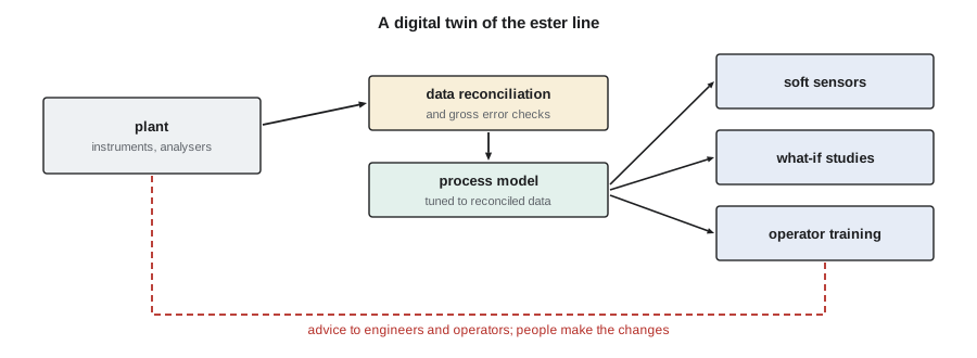
A digital twin, in process engineering, is a model kept continuously in step with a running plant by feeding it reconciled data. The term is used loosely, but a working twin has the parts in the figure: data from the plant, reconciliation and fault checks, a model tuned to the reconciled data, and applications that use it, such as soft sensors, performance monitoring, what-if studies and training. The tuning step adjusts a few parameters, such as exchanger fouling factors, tray efficiencies or a catalyst activity, so that the model matches the plant as it is now. The adjusted parameters are themselves useful: a fouling factor rising week by week tells maintenance when to clean an exchanger.
Wren's view of the twin is practical. It should tell her operators what the plant is doing that they cannot see directly, and what is likely to happen if they make a change. It should not make changes itself without the control system's normal safeguards and the operators' knowledge. Kingfisher Bioenergy's policy for its existing plant is that models give advice, and advanced control applications that act on the plant are designed, tested and managed like any other part of the control system. The twin of the ester line will follow the same rule.
| Application | Model type | Data needed | Main risk |
|---|---|---|---|
| Relief and upset studies | Steady state and dynamic | Equipment data | Simplifications not on the conservative side |
| Pinch and heat recovery | Steady state | Stream temperatures and duties | Base case not representative |
| Data reconciliation | Balances | Measurements and uncertainties | Hidden gross errors |
| Soft sensor | Fitted from model or data | Fast measurements | Use outside the fitted range |
| Surrogate model | Fitted to rigorous model | Rigorous results over a range | Extrapolation |
| Digital twin | Rigorous, tuned online | Reconciled plant data | Drift; trusting it without checks |
Common mistakes
MistakeUsing raw plant data to tune a model.
InsteadReconcile first and check for gross errors.
MistakeUsing a soft sensor or surrogate outside its fitted range.
InsteadRecord the range and flag predictions outside it.
MistakeAssuming the model's relief timing is conservative.
InsteadCheck each simplification for the direction of its error.
MistakeLetting a model change the plant without safeguards.
InsteadModels advise; any application that acts is managed as part of the control system.
Summary and key terms
- Models supply process safety information and check changes and upset scenarios.
- Model duties and temperatures support pinch analysis and energy monitoring.
- Data reconciliation adjusts measurements by weighted least squares to satisfy balances and detects gross errors.
- Soft sensors and surrogates give fast estimates, valid only within their fitted ranges.
- A digital twin is a model kept in step with plant data, used to advise engineers and operators.
- Data reconciliation
- Adjustment of measurements, weighted by their uncertainty, to satisfy model balances.
- Gross error
- A measurement error much larger than the stated uncertainty, such as a failed meter.
- Global test
- A chi-squared test of reconciliation residuals for the presence of gross errors.
- Soft sensor
- An estimate of a hard-to-measure variable from other measurements.
- Surrogate model
- A fast approximate model fitted to the results of a rigorous model.
- Digital twin
- A process model kept continuously in step with a running plant.
Practice problems
Work each problem on paper first, then reveal the answer to check.
How does reconciliation weight measurements?
Show answer
Inversely by their variance, so precise meters move least.
What did the global test give for the decanter data?
Show answer
0.23 against a critical value of 3.84: no gross error.
What happens with the aqueous meter reading 560 kg/h?
Show answer
The statistic rises to 4.11 and flags a possible gross error.
Why should the surrogate's 1,133 kW not be trusted?
Show answer
It is outside the range of reflux used for the fit.
What does a rising fouling factor in a twin tell maintenance?
Show answer
An exchanger is fouling and will need cleaning.
What is Kingfisher Bioenergy's rule on models acting on the plant?
Show answer
Models advise; acting applications are managed as part of the control system.
Lesson quiz · 5 questions
Score 60% or more to complete this lesson.
Create a free account to save your progress, take quizzes and earn a certificate.