
CHE-460 · Lesson 3 of 12 · 21 min
Choosing a thermodynamic method
The two flagged items in Theo's validation table both pointed at the decanter. Before touching any efficiency or heat loss, Ingrid asks him to revisit the most important decision in any simulation: the thermodynamic method. Every unit model in the flowsheet calls the property method thousands of times, for K-values, enthalpies, densities and phase splits. If the method is wrong, every unit is wrong in a consistent way, and no amount of convergence will fix it. Simulator vendors and experienced practitioners agree that a poor choice of property method is among the most common causes of a bad simulation.
A thermodynamic method, sometimes called a property package or fluid package, is a set of models for the properties of mixtures. For vapour-liquid equilibrium, the central question is how to calculate the fugacity of each component in each phase. There are two broad approaches. Equation-of-state methods describe both phases with one equation relating pressure, volume and temperature, such as Peng-Robinson or Soave-Redlich-Kwong. Activity coefficient methods describe the liquid with a model for the excess Gibbs energy, such as Wilson, NRTL, UNIQUAC or van Laar, and the vapour with an ideal gas or a simple equation of state.
A decision tree
Practitioners use a decision tree based on the type of components and the pressure. Mixtures of hydrocarbons and light gases, such as those in gas processing and refining, are well described by cubic equations of state at any pressure. Mixtures of polar or hydrogen-bonding components, such as alcohols, acids, water and esters, are strongly non-ideal in the liquid, and at low to moderate pressure an activity coefficient model is the usual choice. If there are binary interaction parameters fitted to data for the important pairs, the model will be good; if not, a group contribution method such as UNIFAC can estimate them, with less accuracy. At high pressure with polar components, specialized equations of state with advanced mixing rules are used. Electrolytes and polymers need their own methods.
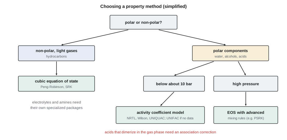
The ester line is a textbook case for an activity coefficient model. The pressure is near atmospheric, the components are all polar, and they form azeotropes: ethanol-water, ethyl acetate-ethanol, ethyl acetate-water, and a ternary azeotrope of all three. Ethyl acetate and water are only partly miscible, which is why the decanter works. NRTL and UNIQUAC can represent both vapour-liquid and liquid-liquid equilibrium; the Wilson model cannot predict two liquid phases and so is unsuitable for the decanter. Acetic acid adds a complication. It associates into dimers in the vapour, so the vapour is far from ideal even at low pressure. Simulators offer a vapour model that accounts for this association, often based on the Hayden-O'Connell correlation, and it should be used whenever acetic acid is present.
How much the choice matters
To show Theo the size of the effect, Ingrid has him calculate the ethanol-water bubble point curve at atmospheric pressure twice: once assuming an ideal liquid, and once with the van Laar model and the parameters fitted in CHE-320. The code below does it with the Antoine equation for vapour pressure.
# Choosing a thermodynamic method: ideal (Raoult) versus van Laar for ethanol (1) + water (2) at 101.325 kPa,
# and regressing van Laar parameters from laboratory activity coefficients (illustrative data)
import math
ANT = {1: (8.20417, 1642.89, 230.300), 2: (8.07131, 1730.63, 233.426)}   # log10 P[mmHg], T[C]
def psat(i, T):
    A, B, C = ANT[i]; return 10 ** (A - B / (C + T)) * 0.133322   # kPa
def vanlaar(x1, A12, A21):
    x2 = 1 - x1
    if x1 in (0.0, 1.0):
        return (math.exp(A12) if x1 == 0 else 1.0), (math.exp(A21) if x1 == 1 else 1.0)
    d = A12 * x1 + A21 * x2
    return math.exp(A12 * (A21 * x2 / d) ** 2), math.exp(A21 * (A12 * x1 / d) ** 2)
def bubble(x1, model, P=101.325):
    lo, hi = 50.0, 110.0
    for _ in range(60):
        T = 0.5 * (lo + hi)
        g1, g2 = model(x1)
        s = x1 * g1 * psat(1, T) + (1 - x1) * g2 * psat(2, T)
        lo, hi = (T, hi) if s < P else (lo, T)
    y1 = x1 * g1 * psat(1, T) / P
    return T, y1
ideal = lambda x: (1.0, 1.0)
vl = lambda x: vanlaar(x, 1.672, 0.930)
print(" x1     T ideal  y1 ideal |  T van Laar  y1 van Laar")
for x1 in (0.02, 0.05, 0.10, 0.30, 0.60, 0.89):
    Ti, yi = bubble(x1, ideal); Tv, yv = bubble(x1, vl)
    print(f"{x1:5.2f}   {Ti:6.1f}   {yi:7.3f}  |   {Tv:6.1f}     {yv:7.3f}")
print()
# Regression: van Laar written as x1 x2 / (gE/RT) = 1/A12 + x1 (1/A21 - 1/A12), a straight line in x1
lab = [(0.05, 4.12, 1.00), (0.10, 3.13, 1.04), (0.20, 2.24, 1.09), (0.35, 1.52, 1.26),
       (0.50, 1.26, 1.45), (0.65, 1.08, 1.75), (0.80, 1.04, 2.04)]      # x1, gamma1, gamma2 (illustrative)
X, Y = [], []
for x1, g1, g2 in lab:
    gE = x1 * math.log(g1) + (1 - x1) * math.log(g2)
    X.append(x1); Y.append(x1 * (1 - x1) / gE)
n = len(X); mx = sum(X) / n; my = sum(Y) / n
b = sum((a - mx) * (c - my) for a, c in zip(X, Y)) / sum((a - mx) ** 2 for a in X)
a = my - b * mx
A12 = 1 / a; A21 = 1 / (a + b)
print(f"fitted van Laar A12 = {A12:.3f}, A21 = {A21:.3f}")
rms = math.sqrt(sum((math.log(vanlaar(x1, A12, A21)[0]) - math.log(g1)) ** 2 for x1, g1, g2 in lab) / n)
print(f"RMS error in ln(gamma1) over the data: {rms:.3f}")x1 T ideal y1 ideal | T van Laar y1 van Laar 0.02 99.3 0.044 | 95.1 0.178 0.05 98.3 0.105 | 90.6 0.323 0.10 96.8 0.200 | 86.6 0.440 0.30 91.3 0.492 | 81.7 0.583 0.60 84.9 0.774 | 79.2 0.703 0.89 79.9 0.949 | 78.2 0.892 fitted van Laar A12 = 1.633, A21 = 0.965 RMS error in ln(gamma1) over the data: 0.021
The differences are dramatic. At 10 % ethanol in the liquid, the ideal model predicts a bubble point of 96.8 °C and an ethanol vapour fraction of 0.20. The van Laar model, which matches published data closely, predicts 86.6 °C and 0.44. An ideal model would design a stripper with far too few stages and far too much reboiler duty, and it would miss the azeotrope near 89 mol % ethanol completely. At the dilute end, where the stripper works, the activity coefficient of ethanol is about five, and the ideal model is wrong by that factor.
Worked problem
Bubble point by hand
Estimate the bubble point pressure at 80 °C of a liquid with \(x_{1} = 0.30\) ethanol and \(x_{2} = 0.70\) water, using \(\gamma_{1} = 2.0\), \(\gamma_{2} = 1.15\), \(P_{1}^{\text{sat}} = 108.3\) kPa and \(P_{2}^{\text{sat}} = 47.4\) kPa.
Show solution
- With modified Raoult's law, \(P = x_{1}\gamma_{1}P_{1}^{\text{sat}} + x_{2}\gamma_{2}P_{2}^{\text{sat}}\).
- Ethanol term: \(0.30 \times 2.0 \times 108.3 = 65.0\) kPa.
- Water term: \(0.70 \times 1.15 \times 47.4 = 38.2\) kPa.
- Sum: \(P = 103.1\) kPa; vapour fraction of ethanol \(y_{1} = 65.0 / 103.1 = 0.63\).
Answer: About 103 kPa, so the mixture boils just above 80 °C at atmospheric pressure, with a vapour of about 63 % ethanol. The ideal model would give about 66 kPa and predict that the liquid is well below its boiling point.
Binary interaction parameters and regression
An activity coefficient model is only as good as its binary interaction parameters. Simulator data banks contain parameters for many common pairs, regressed from published data, and often say which data set and temperature range they came from. Theo checks each pair in the ester system. Ethanol-water, ethanol-ethyl acetate and acid-water are well represented, with parameters fitted to vapour-liquid data at atmospheric pressure. The ethyl acetate-water pair has two sets: one fitted to vapour-liquid data, and one to liquid-liquid data. The decanter needs the second. The base case had used the first, which explains the low aqueous flow.
Where data for a pair is missing or doubtful, the engineer can regress new parameters from laboratory measurements. Dev, the Kingfisher Bioenergy laboratory chemist, measures seven vapour-liquid equilibrium points for ethanol-water at atmospheric pressure as a check on the method. The second part of the code fits the van Laar parameters by linear least squares, using the fact that the van Laar equation can be rearranged into a straight line. The fitted values, 1.633 and 0.965, are close to the published 1.672 and 0.930, and the root-mean-square error in the logarithm of the activity coefficient is about 0.02. Simulators provide regression tools that do the same for NRTL and UNIQUAC parameters, with statistics on the fit.
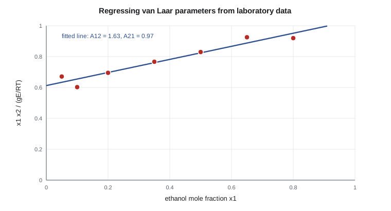
A good fit to the data used is not the whole test. Ingrid asks two further questions. Is the model consistent with other data, such as infinite dilution activity coefficients or azeotrope compositions, that were not used in the fit? And does it predict any false phase splits, such as a second liquid phase where there should be none? Activity coefficient parameters fitted to vapour-liquid data sometimes predict liquid-liquid splitting at conditions outside the fitted range. A quick check is to have the simulator calculate the phase envelope of each binary at the operating temperatures and look for unexpected regions.
Enthalpy, density and transport properties
Phase equilibrium is not the only output of a property method. Every energy balance needs enthalpies, and the property method supplies them: ideal-gas heat capacities for each component, heats of vaporization, and an excess enthalpy for the liquid mixture if the activity coefficient model is temperature-dependent. For the ester line the heats of mixing are small compared with the latent heats, and errors of a few per cent in them hardly move the duties. The latent heats are another matter. The reboiler duty of the ester column is almost all latent heat, so Theo checks the simulator's heat of vaporization for ethyl acetate and ethanol against published values at the column temperatures. They agree within one per cent.
Equipment sizing also needs liquid density, viscosity, thermal conductivity and surface tension. Simulators estimate these from correlations that are usually adequate for organic liquids. Hydraulic design of trays and packing, and heat exchanger rating, depend on them, and the contractor's equipment specialists will often override the simulator's values with their own data. Theo makes a note to compare the densities and viscosities in the two models, since a 10 % difference in viscosity can change a calculated exchanger coefficient noticeably.
Thermodynamic consistency and data sources
Experimental vapour-liquid data can be checked for thermodynamic consistency: the Gibbs-Duhem equation requires the activity coefficients of the components in a mixture to be related, and data that violate it beyond a tolerance contain errors. Data compilations and some simulators apply consistency tests and flag doubtful sets. Reliable compilations, such as the DECHEMA data series and the data banks distributed with simulators, have been evaluated in this way. The United States National Institute of Standards and Technology also offers tools that evaluate thermophysical data dynamically. Theo records in the model log which data set each parameter came from, so that a later engineer can trace it.
| Pair | Behaviour | Data used for parameters |
|---|---|---|
| Ethanol, water | Positive deviation, minimum-boiling azeotrope | Vapour-liquid, atmospheric |
| Ethyl acetate, ethanol | Minimum-boiling azeotrope | Vapour-liquid, atmospheric |
| Ethyl acetate, water | Partial miscibility, heterogeneous azeotrope | Liquid-liquid, 20 to 60 °C |
| Acetic acid, water | Nearly ideal liquid; vapour dimerization | Vapour-liquid with association |
| Acetic acid, ethyl acetate | Moderate deviation | Vapour-liquid; less certain |
With the liquid-liquid parameter set for ethyl acetate-water, and the association model for the acid in the vapour, Theo reruns the validation. The decanter aqueous flow moves from 8.8 % low to 2.4 % low, and the reboiler duty from 6.5 % low to 3.1 % low, both now within tolerance. Fixing the cause, rather than tuning, has improved two quantities at once.
Common mistakes
MistakeAccepting the simulator's default property method.
InsteadChoose the method from the components, pressure and available data.
MistakeUsing the Wilson model for a system with two liquid phases.
InsteadUse NRTL or UNIQUAC, which can predict liquid-liquid splits.
MistakeIgnoring acid dimerization in the vapour.
InsteadUse an association model for the vapour whenever carboxylic acids are present.
MistakeUsing vapour-liquid parameters for a decanter.
InsteadUse parameters fitted to liquid-liquid data for liquid-liquid units.
Summary and key terms
- The thermodynamic method is the most important choice in a simulation.
- Equations of state suit hydrocarbons and gases; activity coefficient models suit polar mixtures at low pressure.
- Activity coefficient models need binary interaction parameters fitted to good data for the important pairs.
- Parameters can be regressed from laboratory data, and should be checked against independent data and for false phase splits.
- Acetic acid needs a vapour association model; decanters need liquid-liquid parameters.
- Property method
- The set of models a simulator uses to calculate mixture properties and phase equilibrium.
- Activity coefficient
- A factor correcting the ideal-solution fugacity of a liquid component for non-ideal interactions.
- Equation of state
- A relation among pressure, volume and temperature used to calculate fugacities in both phases.
- Binary interaction parameter
- A fitted constant describing the interaction of a pair of components in a mixture model.
- UNIFAC
- A group contribution method that estimates activity coefficients from molecular structure.
- Thermodynamic consistency
- Agreement of measured data with the Gibbs-Duhem relation.
Practice problems
Work each problem on paper first, then reveal the answer to check.
Which type of method suits a hydrocarbon gas mixture at 60 bar?
Show answer
A cubic equation of state such as Peng-Robinson.
Why is the Wilson model unsuitable for the decanter?
Show answer
It cannot predict two liquid phases.
At 10 % ethanol, what are the ideal and van Laar bubble points?
Show answer
About 96.8 °C ideal and 86.6 °C with van Laar.
What vapour model should be used when acetic acid is present?
Show answer
One that accounts for association, such as one based on Hayden-O'Connell.
Name two checks on regressed parameters beyond goodness of fit.
Show answer
Agreement with independent data, and no false phase splits.
What happened to the validation after the thermodynamic fix?
Show answer
The aqueous flow and reboiler duty errors fell within tolerance.
Lesson quiz · 5 questions
Score 60% or more to complete this lesson.
Create a free account to save your progress, take quizzes and earn a certificate.