
CHE-460 · Lesson 2 of 12 · 22 min
Building and validating a flowsheet
Theo's first task is to lay out the owner's model of the ester line so that it can be compared, stream by stream, with the contractor's heat and material balance. The line, as sanctioned in CHE-446, takes fresh acetic acid and ethanol, mixes them with recycled acid and ethanol, and reacts them in a fixed-bed pre-reactor over an acid ion-exchange resin. The reactor effluent goes to a reactive distillation column where the reaction continues and the light ester-ethanol-water azeotrope goes overhead. The overhead condenses and splits in a decanter into an ester-rich organic phase and a water-rich aqueous phase. The organic phase feeds the ester column, which takes high-purity ethyl acetate from the bottom and returns its distillate to the decanter. A stripper recovers ethanol from the aqueous phase before the water goes to treatment, and the recovered ethanol and unreacted acid are recycled.
A flowsheet is the simulator's picture of that process: a set of unit operation blocks joined by material and energy streams. It looks like a process flow diagram, and it should be drawn to match the plant's diagram tag for tag, so that anyone can find a stream in the model from its number on the drawing. But a flowsheet is not a drawing. Each block is a set of equations, each stream a set of variables, and the arrangement determines the order in which a sequential-modular simulator calculates them.
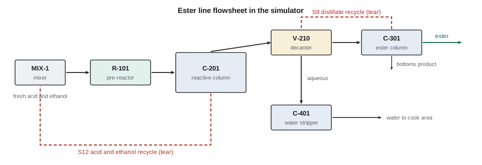
Laying out the flowsheet
Ingrid recommends building in stages, and getting each stage to converge before adding the next. Theo starts with the feed streams and the mixer, then the pre-reactor with a simple fixed conversion, then the reactive column as an ordinary column with a reaction, then the decanter, and only last the ester column and the stripper. At each stage he checks the overall balance. When a stage fails, he knows the fault lies in what he just added. Building the whole flowsheet at once and pressing run is the most common way to produce a model that will not converge and gives no clue why.
The components come first. For the ester line they are acetic acid, ethanol, ethyl acetate and water, plus the trace impurities that matter for product quality: n-propanol from the ethanol feed, and the small amount of diethyl ether that the resin can form. Each component needs pure-component properties: molecular weight, critical constants, vapour pressure, heat capacity, heat of vaporization and density. Simulators supply these from data banks. Theo checks the vapour pressure of each main component against the data in CHE-320 at the operating temperatures, because a few per cent error in vapour pressure moves the column profile significantly.
Next come the feed streams. Each needs a flow, a composition, and two of temperature, pressure and vapour fraction. Theo enters the fresh feeds from the design basis: acetic acid at 99.85 % with water as the balance, and ethanol at 99.5 % with water and a trace of propanol. Then the unit blocks, one per piece of equipment, each with its specifications. For the first pass he uses simple blocks: a stoichiometric reactor with a fixed conversion, shortcut columns and a component splitter for the decanter. Rigorous models replace them once the flowsheet converges.
Stream tables
The main output of a steady-state model is the stream table: for each stream, its flow, composition, temperature, pressure and phase. It is the heat and material balance that engineers use to size equipment, and the first thing a checker reads. A stream table should always close: the sum of the mass flows into any unit, and into the whole plant, should equal the sum out, to the rounding of the numbers shown. Mole flows need not close across a reactor, because reactions can change the number of moles, but for esterification the moles are conserved: one acid and one ethanol give one ester and one water.
# Build a stream table for the front of the ester line, then compare the model with plant test data
MW = {"acid": 60.05, "ethanol": 46.07, "ester": 88.11, "water": 18.02}
fresh = {"acid": 26.4, "ethanol": 26.3, "ester": 0.0, "water": 0.4}      # kmol/h
recycle = {"acid": 13.8, "ethanol": 21.9, "ester": 4.1, "water": 6.2}    # kmol/h, first guess
def mix(*streams):
    out = {k: 0.0 for k in MW}
    for s in streams:
        for k, v in s.items(): out[k] += v
    return out
def react(s, X_acid):
    # CH3COOH + C2H5OH -> CH3COOC2H5 + H2O, conversion based on acid
    r = X_acid * s["acid"]
    return {"acid": s["acid"] - r, "ethanol": s["ethanol"] - r, "ester": s["ester"] + r, "water": s["water"] + r}
def kgh(s): return sum(s[k] * MW[k] for k in s)
S1 = mix(fresh, recycle)
S2 = react(S1, 0.652)
print(f"{'stream':12s}{'acid':>8s}{'ethanol':>9s}{'ester':>8s}{'water':>8s}{'kmol/h':>9s}{'kg/h':>9s}")
for name, s in (("fresh", fresh), ("recycle", recycle), ("S1 mixed", S1), ("S2 reactor", S2)):
    print(f"{name:12s}" + "".join(f"{s[k]:8.2f}" if k != "ethanol" else f"{s[k]:9.2f}" for k in MW) + f"{sum(s.values()):9.2f}{kgh(s):9.0f}")
print(f"mass in {kgh(S1):.0f} kg/h, mass out of reactor {kgh(S2):.0f} kg/h (closes: {abs(kgh(S1) - kgh(S2)) < 0.5})")
print()
# Validation against a plant test run on the pilot unit (illustrative measurements)
tags = [  # (tag, model, measured, tolerance %)
    ("reactor outlet T, C",          82.6, 81.9, 2),
    ("ester in S2, mass %",          round(S2["ester"] * MW["ester"] / kgh(S2) * 100, 1), 50.6, 5),
    ("reactive column top T, C",     70.4, 70.9, 2),
    ("ester column reboiler, kW",     952, 1018, 5),
    ("ester product, kg/h",          2300, 2276, 3),
    ("decanter aqueous, kg/h",        640,  702, 5),
    ("stripper bottoms ethanol, ppm",  80,  145, 50),
]
for tag, m, p, tol in tags:
    err = (m - p) / p * 100
    flag = "ok" if abs(err) <= tol else "CHECK"
print(f"{tag:32s} model {m:8.1f} plant {p:8.1f} error {err:+6.1f} % tolerance {tol:>3d} % {flag.lower()}")stream acid ethanol ester water kmol/h kg/h fresh 26.40 26.30 0.00 0.40 53.10 2804 recycle 13.80 21.90 4.10 6.20 46.00 2311 S1 mixed 40.20 48.20 4.10 6.60 99.10 5115 S2 reactor 13.99 21.99 30.31 32.81 99.10 5115 mass in 5115 kg/h, mass out of reactor 5115 kg/h (closes: True) reactor outlet T, C model 82.6 plant 81.9 error +0.9 % tolerance 2 % ok ester in S2, mass % model 52.2 plant 50.6 error +3.2 % tolerance 5 % ok reactive column top T, C model 70.4 plant 70.9 error -0.7 % tolerance 2 % ok ester column reboiler, kW model 952.0 plant 1018.0 error -6.5 % tolerance 5 % check ester product, kg/h model 2300.0 plant 2276.0 error +1.1 % tolerance 3 % ok decanter aqueous, kg/h model 640.0 plant 702.0 error -8.8 % tolerance 5 % check stripper bottoms ethanol, ppm model 80.0 plant 145.0 error -44.8 % tolerance 50 % ok
The table shows the fresh feed of 53.1 kmol/h mixing with 46.0 kmol/h of recycle to give a reactor feed of 99.1 kmol/h. At the design conversion of 65.2 % of the acid, the reactor effluent carries about 30.3 kmol/h of ester and 32.8 kmol/h of water. The mass flows in and out agree. A table like this, worked by hand or in a few lines of code, is the best possible check on the simulator. If the simulator's numbers for the same streams are different, either the simulator has been given a different input or the hand calculation has a mistake, and finding out which is always instructive.
Validation
Validation means comparing the model with measurements and deciding whether the agreement is good enough for the model's purpose. For a new plant there is no plant data, so Theo uses the next best thing: the licensor's report from a demonstration unit that ran the same reactive column and decanter at one-tenth scale for several months. The report gives measured temperatures, compositions, flows and duties for a steady run. Theo sets the model's feeds and specifications to the run conditions and compares.
Each comparison needs a tolerance, decided in advance and based on how well the quantity can be measured and how much the purpose depends on it. Temperatures are measured to about a degree, so a model temperature within a few per cent is acceptable. Flows from calibrated meters may be good to one or two per cent. Duties are calculated from steam flow and pressure, which adds uncertainty, so a tolerance of five per cent is usual. Trace compositions from laboratory analysis may be uncertain by tens of per cent, and the tolerance for them is wide.
In the validation table, most quantities agree within tolerance. Two do not: the reboiler duty is 6.5 % low in the model and the decanter aqueous flow is 8.8 % low. These are flagged, not ignored. Both point in the same direction: the model sends a little less water to the aqueous phase, so less liquid circulates, and less heat is needed. The likely cause is the liquid-liquid equilibrium in the decanter, which depends on parameters for the ester-water pair that were fitted to data at a different temperature. Theo notes it and returns to it in lesson 3, where the thermodynamic method is chosen properly. The trace ethanol in the stripper bottoms differs by 45 %, but the tolerance for a trace concentration from laboratory analysis is 50 %, and the error is accepted.
| Quantity | Typical measurement uncertainty | Typical validation tolerance |
|---|---|---|
| Temperature | 0.5 to 1 K | 1 to 3 % |
| Pressure | 0.5 % | 2 % |
| Flow from a calibrated meter | 1 to 2 % | 3 % |
| Major composition by laboratory analysis | 1 to 3 % | 3 to 5 % |
| Heat duty from steam flow | 3 to 5 % | 5 % |
| Trace composition | 10 to 30 % | 30 to 50 % |
Worked problem
Checking a validation result
A model predicts a column top temperature of 70.4 °C. The demonstration unit measured 70.9 °C. The tolerance is 2 %. Is the model acceptable on this point?
Show solution
- Error = (70.4 − 70.9) / 70.9 = −0.7 %.
- The magnitude 0.7 % is less than 2 %.
- Note also that a 0.5 K difference is within the accuracy of a typical thermocouple and transmitter.
- So the model agrees with the measurement on this point.
Answer: Yes. The error of −0.7 % is within tolerance, and in absolute terms is within measurement accuracy.
Common causes of poor agreement
When a model disagrees with data, the fault lies in one of a short list of places. The feed may be wrong: a composition entered in mass fractions when the simulator expects mole fractions is a classic mistake. The thermodynamic method may be unsuitable, or its parameters may have been fitted outside the operating range. A column may be modelled with too many or too few equilibrium stages, or with the wrong efficiency. Heat losses, ignored in the model, may be significant in a small pilot unit. And the data itself may be wrong: a meter out of calibration, a sample taken at the wrong time, a plant not quite at steady state. Lesson 11 shows how data reconciliation detects bad measurements.
Ingrid's advice is to fix causes, not symptoms. It is always possible to adjust an efficiency or a heat loss until a model matches one data set. A model tuned that way will match that one run and fail on the next. A model whose thermodynamics and equipment descriptions are right, with few adjusted parameters, will predict new conditions well, which is the whole point of having it.
Units deserve a word of their own. Simulators let the user choose units for every quantity, and a model passed between engineers in different offices may switch from kilomoles per hour to pounds per hour, or from kilopascals absolute to pounds per square inch gauge, without anyone noticing. The contractor for the expansion reports pressures in bar gauge; Kingfisher Bioenergy's operating procedures use kilopascals absolute. Theo sets the model to the plant's units, records the choice at the top of the model log, and converts the contractor's numbers explicitly when he compares. A gauge-absolute mix-up of about 101 kPa is small for a high-pressure unit and large for a column running near atmospheric pressure, where it can change the boiling temperatures by twenty kelvin.
Documenting the base case
Once the flowsheet converges and validates, Theo saves it as the base case and records it in the model log: version, date, the list of components and data sources, the property method, each unit with its specifications, the convergence settings, and the validation table with its two flagged items. Every later study starts from a copy of the base case, so that the base remains a fixed reference. When the contractor issues their heat and material balance, Theo compares it with his base case, and the differences become a list of questions for the next design review.
Common mistakes
MistakeBuilding the whole flowsheet before running any of it.
InsteadBuild and converge in stages so faults are easy to locate.
MistakeEntering mass fractions where the simulator expects mole fractions.
InsteadCheck the basis of every feed entry.
MistakeTuning efficiencies until one data set matches.
InsteadFix the thermodynamics and equipment description first; adjust as few parameters as possible.
MistakeNot deciding validation tolerances in advance.
InsteadSet tolerances from measurement uncertainty and purpose before comparing.
Summary and key terms
- A flowsheet is a set of unit blocks and streams that should match the plant's diagram tag for tag.
- Build in stages, converging each before adding the next, and start with simple models.
- The stream table is the heat and material balance; it must close on mass.
- Validation compares model and data against tolerances set from measurement uncertainty and purpose.
- Investigate and fix causes of disagreement rather than tuning parameters to one data set.
- Flowsheet
- The arrangement of unit blocks and streams that represents a process in a simulator.
- Stream table
- A table of flows, compositions, temperatures, pressures and phases for each stream.
- Base case
- The converged, validated model saved as the reference for all later studies.
- Tolerance
- The largest model error accepted for a quantity during validation.
- Shortcut model
- A simple unit model, such as fixed conversion or fixed split, used early in model building.
Practice problems
Work each problem on paper first, then reveal the answer to check.
Why should a flowsheet be built in stages?
Show answer
So that each fault can be traced to the part just added.
Do mole flows close across the esterification reactor?
Show answer
Yes, because one acid and one ethanol give one ester and one water.
The model's reboiler duty is 6.5 % below measured, with a 5 % tolerance. What do you do?
Show answer
Flag it and look for a cause, such as liquid-liquid equilibrium parameters or heat losses.
Why are tolerances for trace compositions wide?
Show answer
Laboratory analysis of trace components is uncertain by tens of per cent.
What is the risk of tuning a model to one data set?
Show answer
It matches that run but predicts other conditions poorly.
What should be recorded for the base case?
Show answer
Version, components and sources, property method, unit specifications, convergence settings and validation.
Lesson quiz · 5 questions
Score 60% or more to complete this lesson.
Create a free account to save your progress, take quizzes and earn a certificate.