
CHE-374 · Lesson 8 of 12 · 22 min
PID tuning
Theo now has everything he needs to retune tray 13: a model, \(K = 0.90\) °C per percent, \(\tau = 6.5\) min and \(\theta = 2.5\) min; an ultimate gain of 5.27 %/°C at a period of 8.8 min; and a working valve. What he lacks is a reason to prefer one set of numbers over another. Dozens of tuning rules exist. They were derived for different purposes, by different people, with different ideas of what good control means, and applied blindly they can give settings that differ by a factor of three. This lesson compares the rules that matter on the same loop, and shows how to choose.
What good tuning means
A tuning is judged on several things at once. Set-point tracking measures how quickly and smoothly the loop follows a new set point, and is summarized by overshoot and settling time. Load rejection measures how far the measurement moves after a disturbance and how quickly it recovers, summarized by the peak deviation and the integral of absolute error, IAE. Robustness measures how much the process can change before the loop misbehaves, summarized by the gain and phase margins of lesson 7 or by the maximum sensitivity \(M_s\). Valve wear and noise depend on how hard the output moves. These goals conflict: the fastest load rejection comes from aggressive settings that cost robustness. In chemical plants, where most loops face disturbances more often than set-point changes and where process conditions drift, robustness usually wins.
Ziegler-Nichols
In 1942 Ziegler and Nichols published rules based on a closed-loop test: raise the proportional gain until the loop oscillates steadily, note \(K_u\) and \(P_u\), and set a PI controller to \(K_c = 0.45K_u\), \(T_i = P_u/1.2\), or a PID to \(K_c = 0.6K_u\), \(T_i = P_u/2\), \(T_d = P_u/8\). The rules aim at a quarter-decay ratio. They are historically important and give a fast response to load, but they are aggressive. On tray 13 the Ziegler-Nichols PI settings, \(K_c = 2.37\) and \(T_i = 7.3\) min, overshoot a set-point step by 27 %, with \(M_s = 2.3\). Bringing a running column to the edge of instability to measure \(K_u\) is also not something most plants allow; it is usually estimated from a step-test model, as Theo did in lesson 7, or by relay feedback, an automatic test that switches the output between two limits and reads the ultimate period from the resulting oscillation.
Cohen-Coon
Cohen and Coon, in 1953, derived open-loop rules from an FOPDT model, also aiming at quarter decay. They allow for the ratio \(\theta/\tau\) more carefully than Ziegler-Nichols, but for moderate ratios they are even more aggressive. On tray 13 they give \(K_c = 2.69\) and \(T_i = 4.7\) min, with 62 % overshoot and \(M_s = 3.4\). Few practitioners use them today except for very lag-dominant processes.
IMC and lambda tuning
Internal model control, developed in the 1980s, approaches tuning from a different angle: choose the closed-loop response you want, and derive the controller that produces it from the process model. For an FOPDT process, asking for a first-order closed-loop response with time constant \(\lambda\) gives, after approximations, a PI controller:
The single tuning parameter \(\lambda\) sets the speed. A small \(\lambda\) is fast and less robust; a large one is slow and very robust. Lambda tuning is popular in the pulp and paper and chemical industries because it is easy to explain, gives no overshoot on set-point changes and lets an engineer set loops in a unit to coordinated speeds. With \(\lambda = \tau = 6.5\) min, tray 13 gets \(K_c = 0.80\) and \(T_i = 6.5\) min: no overshoot, \(M_s = 1.28\), but sluggish load rejection with a peak deviation of 0.94 °C and an IAE nearly three times that of Ziegler-Nichols.
SIMC: simple and robust
Skogestad's SIMC rules, published in 2003, modify IMC tuning so that load rejection is not sacrificed when \(\tau\) is large. For an FOPDT process with desired closed-loop time constant \(\tau_c\):
The recommended default is \(\tau_c = \theta\), which gives good robustness, typically a gain margin around 3 and a phase margin around 45° to 60°. For tray 13 that is \(K_c = 6.5/(0.9 \times 5) = 1.44\) %/°C and \(T_i = 6.5\) min. The integral time limit only becomes active for lag-dominant or integrating processes, where it stops the integral action from becoming so slow that load disturbances linger.
# PI(D) tuning rules compared on the tray-temperature loop (K 0.90 degC/%, tau 6.5 min, theta 2.5 min)
import math, random
def fopdt_step(K, tau, theta, t):
    # response of K e^(-theta s)/(tau s + 1) to a unit step at t = 0
    return 0.0 if t < theta else K * (1 - math.exp(-(t - theta) / tau))
class Plant:
    # first- or second-order lag with dead time, stepped with Euler at a small dt
    def __init__(self, K, tau1, theta, dt, tau2=0.0):
        self.K, self.t1, self.t2, self.dt = K, tau1, tau2, dt
        self.buf = [0.0] * max(1, int(round(theta / dt)))
        self.x1 = 0.0; self.x2 = 0.0
    def step(self, u):
        self.buf.append(u); ud = self.buf.pop(0)
        self.x1 += self.dt * (self.K * ud - self.x1) / self.t1
        if self.t2 > 0:
            self.x2 += self.dt * (self.x1 - self.x2) / self.t2
            return self.x2
        return self.x1
def loop(K, tau, theta, Kc, Ti, Td=0.0, tend=60.0, dt=0.01, sp=1.0, load=0.0, t_load=0.0,
         umin=-1e9, umax=1e9, antiwindup=True, tau2=0.0):
    # PI(D) control of an FOPDT (or SOPDT) plant; derivative acts on the measurement.
    # A load enters at the plant input at t_load. Returns lists of t, y, u.
    p = Plant(K, tau, theta, dt, tau2)
    I, ylast, y = 0.0, 0.0, 0.0
    T, Y, U = [], [], []
    n = int(tend / dt)
    for k in range(n):
        t = k * dt
        e = sp - y
        D = -Kc * Td * (y - ylast) / dt if Td > 0 else 0.0
        u_un = Kc * e + I + D
        u = min(umax, max(umin, u_un))
        if Ti > 0:
            if not antiwindup or u == u_un or (u_un > umax and e < 0) or (u_un < umin and e > 0):
                I += Kc * dt / Ti * e
        d = load if t >= t_load else 0.0
        ylast = y
        y = p.step(u + d)
        T.append(t); Y.append(y); U.append(u)
    return T, Y, U
def iae(T, Y, sp, t0=0.0):
    dt = T[1] - T[0]
    return sum(abs(sp - y) * dt for t, y in zip(T, Y) if t >= t0)
def overshoot(Y, sp):
    return max(0.0, (max(Y) - sp) / sp * 100) if sp else 0.0
def settle(T, Y, sp, band=0.05):
    last = T[0]
    for t, y in zip(T, Y):
        if abs(y - sp) > band * abs(sp): last = t
    return last
import cmath
K, tau, th, Ku, Pu = 0.90, 6.5, 2.5, 5.27, 8.8
r = th / tau
rules = [
 ("Ziegler-Nichols PI", 0.45 * Ku, Pu / 1.2, 0.0),
 ("Ziegler-Nichols PID", 0.6 * Ku, Pu / 2, Pu / 8),
 ("Cohen-Coon PI", (tau / (K * th)) * (0.9 + th / (12 * tau)), th * (30 + 3 * r) / (9 + 20 * r), 0.0),
 ("SIMC PI, tau_c = theta", tau / (K * 2 * th), min(tau, 8 * th), 0.0),
 ("lambda PI, lambda = tau", tau / (K * (tau + th)), tau, 0.0),
]
def Ms(Kc, Ti, Td):
    best = 0.0
    for i in range(1, 4000):
        w = 0.0005 * i
        s = 1j * w
        L = K * cmath.exp(-th * s) / (tau * s + 1) * Kc * (1 + 1 / (Ti * s) + Td * s)
        best = max(best, abs(1 / (1 + L)))
    return best
print("rule                       Kc     Ti    Td   overshoot  IAE(sp)  max dev(load)  IAE(load)   Ms")
for name, Kc, Ti, Td in rules:
    T, Y, U = loop(K, tau, th, Kc, Ti, Td, tend=80, sp=1.0)
    T2, Y2, U2 = loop(K, tau, th, Kc, Ti, Td, tend=80, sp=0.0, load=-2.0)
    print(f"{name:24s} {Kc:5.2f} {Ti:5.2f} {Td:4.2f}  {overshoot(Y, 1):7.1f} %  {iae(T, Y, 1):6.2f}   {min(Y2):9.3f}     {iae(T2, Y2, 0):7.2f}   {Ms(Kc, Ti, Td):4.2f}")
# Integral windup: the steam valve sits at 90 % and can open only 10 % more; ask for +8 degC (needs +8.9 %)
Kc, Ti = tau / (K * 2 * th), min(tau, 8 * th)
for aw in (False, True):
    T, Y, U = loop(K, tau, th, Kc, Ti, tend=120, sp=8.0, umin=-70, umax=10, antiwindup=aw)
print(f"anti-windup {'on ' if aw else 'off'}: overshoot {overshoot(Y, 8):.1f} %, valve saturated for {sum(1 for u in U if u >= 10) * 0.01:.1f} min, settles at {settle(T, Y, 8, 0.02):.1f} min")rule Kc Ti Td overshoot IAE(sp) max dev(load) IAE(load) Ms Ziegler-Nichols PI 2.37 7.33 0.00 27.1 % 5.60 -0.739 6.18 2.26 Ziegler-Nichols PID 3.16 4.40 1.10 44.0 % 5.82 -0.590 3.10 2.41 Cohen-Coon PI 2.69 4.67 0.00 62.3 % 8.61 -0.718 5.44 3.42 SIMC PI, tau_c = theta 1.44 6.50 0.00 4.1 % 5.42 -0.816 9.00 1.59 lambda PI, lambda = tau 0.80 6.50 0.00 0.0 % 8.99 -0.941 16.20 1.28 anti-windup off: overshoot 11.3 %, valve saturated for 29.5 min, settles at 45.7 min anti-windup on : overshoot 0.0 %, valve saturated for 3.3 min, settles at 26.7 min
| Rule | Kc (%/°C) | Ti (min) | Set-point overshoot | Peak load deviation | Ms |
|---|---|---|---|---|---|
| Ziegler-Nichols PI | 2.37 | 7.3 | 27 % | 0.74 °C | 2.3 |
| Ziegler-Nichols PID | 3.16 | 4.4 | 44 % | 0.59 °C | 2.4 |
| Cohen-Coon PI | 2.69 | 4.7 | 62 % | 0.72 °C | 3.4 |
| SIMC PI, tau_c = theta | 1.44 | 6.5 | 4 % | 0.82 °C | 1.6 |
| Lambda PI, lambda = tau | 0.80 | 6.5 | 0 % | 0.94 °C | 1.3 |
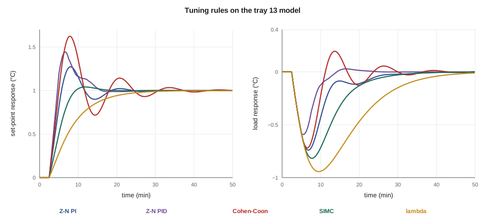
The table makes the trade-off visible. The quarter-decay rules reject the load best, the Ziegler-Nichols PID dipping only 0.59 °C, but they overshoot set-point changes heavily and have maximum sensitivities above 2, so a modest rise in process gain, for instance at a different feed composition, would make them oscillate badly. Lambda tuning with \(\lambda = \tau\) is the most robust and the slowest. SIMC sits between: a small overshoot, a peak load deviation only 0.08 °C worse than Ziegler-Nichols PI, and an \(M_s\) of 1.6. Theo recommends SIMC for tray 13. Malik agrees, adding that for a loop with a known nonlinearity they might choose \(\tau_c\) a little larger than \(\theta\).
Worked problem
SIMC settings for the decanter temperature
A step test on the decanter temperature gives \(K = -1.2\) °C per percent cooling-water valve, \(\tau = 4\) min, \(\theta = 1\) min. Find SIMC PI settings with \(\tau_c = \theta\).
Show solution
- \(K_c = \tau/(|K|(\tau_c + \theta)) = 4/(1.2 \times 2) = 1.67\) %/°C, with the action set from the sign of the gain.
- \(T_i = \min(4,\ 4 \times 2) = 4\) min.
Answer: \(K_c = 1.67\) %/°C and \(T_i = 4\) min; because the gain is negative, a rising temperature must open the cooling valve further.
Derivative action in tuning
The Ziegler-Nichols PID rejects the load faster than any PI tuning, which shows what derivative can do on a lag-dominant loop. The price is noise. The tray temperature's 0.05 °C of noise, passed through a derivative time of 1.1 min and a gain of 3.2, would move the steam valve by several tenths of a percent every few seconds unless filtered. Most temperature loops at Kingfisher Bioenergy run as PI. Derivative is used on a few large thermal loops, such as fired heater outlets, with filtering, and its benefit is checked in the field rather than assumed.
Windup and anti-windup
Every real controller output is limited: a valve cannot open beyond 100 % or close below 0 %. If the controller asks for more than the valve can give, the error persists, and a plain integral term keeps growing. When the error finally changes sign, the inflated integral holds the valve at its limit long after it should have moved, producing a large overshoot. This is integral windup. The code shows it on tray 13 with the steam valve already at 90 % and only 10 % of travel left, when the operator asks for an 8 °C rise that needs 8.9 % more steam. Without protection the valve sits at its limit for nearly half an hour, the temperature overshoots by 11 % and settles only after 46 minutes. With anti-windup, which stops integrating while the output is saturated and the error would push it further, the temperature approaches the set point without overshoot and settles in 27 minutes.
Every DCS PID block includes some form of anti-windup, usually conditional integration or back-calculation. Windup also appears in subtler forms: in cascade loops when the inner loop saturates, lesson 9, and in override schemes where one controller is not in control. Theo learns to check that each block's output limits match the real valve limits.
Bumpless transfer and field practice
When an operator switches a loop from manual to automatic, a well-designed block initializes its integral so that the output does not jump. When tuning is changed online, the output should not jump either. These details, together with set-point ramping and output rate limits, decide whether operators trust a loop. Malik's tuning procedure for the plant is short: confirm the valve works; do a step test; fit an FOPDT model; apply SIMC with \(\tau_c = \theta\), or larger if the process varies; check the margins; test with a small set-point change; watch the loop through at least one real disturbance; record the settings, form, units and model in the loop file.
Theo's new tray 13 settings go in on a Thursday. The next feed change comes the following Monday; the temperature dips 0.6 °C and recovers in under twenty minutes without cycling. Carla leaves the loop in automatic.
Common mistakes
MistakeTuning by quarter decay on a loop whose process gain varies.
InsteadQuarter-decay rules leave little margin; use SIMC or lambda tuning.
MistakeChoosing \(T_i\) much shorter than \(\tau\) to speed up a loop.
InsteadFast integral adds phase lag and oscillation; keep \(T_i\) near \(\tau\) for FOPDT processes.
MistakeIgnoring output limits in a simulation.
InsteadReal valves saturate; check for windup and anti-windup behaviour.
MistakeMeasuring \(K_u\) by driving a production unit to sustained oscillation.
InsteadEstimate it from a model or use a relay test.
Summary and key terms
- Good tuning balances set-point tracking, load rejection, robustness and valve movement.
- Ziegler-Nichols and Cohen-Coon aim at quarter decay and are aggressive, with \(M_s\) of 2.3 to 3.4 on tray 13.
- Lambda tuning sets \(K_c = \tau/(K(\lambda + \theta))\), \(T_i = \tau\); robust but slow on load.
- SIMC with \(\tau_c = \theta\) gives tray 13 \(K_c = 1.44\) %/°C, \(T_i = 6.5\) min, 4 % overshoot and \(M_s = 1.6\).
- Anti-windup removed an 11 % overshoot after the steam valve saturated.
- Integral of absolute error
- The time integral of the magnitude of the error, a measure of control performance.
- Quarter decay
- A response in which each peak is a quarter of the previous one.
- Lambda tuning
- An IMC-based method in which the closed-loop time constant lambda is chosen directly.
- SIMC
- Skogestad's simple IMC-based tuning rules for PI and PID controllers.
- Integral windup
- Growth of the integral term while the output is saturated, causing overshoot.
- Relay test
- An automatic test that finds the ultimate period from a switching output.
- Bumpless transfer
- Switching modes or settings without a jump in controller output.
Practice problems
Work each problem on paper first, then reveal the answer to check.
Find Ziegler-Nichols PI settings for \(K_u = 3\), \(P_u = 12\) min.
Show answer
\(K_c = 1.35\), \(T_i = 10\) min.
Give lambda settings for \(K = 2\), \(\tau = 10\), \(\theta = 2\) min with \(\lambda = 5\) min.
Show answer
\(K_c = 10/(2 \times 7) = 0.71\), \(T_i = 10\) min.
Give SIMC settings for \(K = 0.5\), \(\tau = 20\), \(\theta = 1\) min with \(\tau_c = \theta\).
Show answer
\(K_c = 20/(0.5 \times 2) = 20\), \(T_i = \min(20, 8) = 8\) min.
Why does SIMC cap \(T_i\) at \(4(\tau_c + \theta)\)?
Show answer
So that lag-dominant loops still reject load disturbances in reasonable time.
A loop overshoots badly only after large set-point changes. Suspect what?
Show answer
Windup from output saturation.
What does \(M_s = 3\) imply?
Show answer
Low robustness: the loop is close to instability and amplifies some disturbances.
Lesson quiz · 5 questions
Score 60% or more to complete this lesson.
Create a free account to save your progress, take quizzes and earn a certificate.