
CHE-374 · Lesson 7 of 12 · 23 min
Closed-loop stability and frequency response
The old tuning on the tray 13 loop had a gain of 4 %/°C, and Carla's complaint was that it cycled with a period of about 9 minutes after every feed change. Theo wants to know how close that tuning was to the edge, and how much margin a new tuning should keep. Stability analysis answers both questions. It is also the tool that explains why dead time, more than anything else, limits how hard a chemical process loop can be pushed.
The characteristic equation
Lesson 3 showed that a closed loop's poles are the roots of \(1 + G_{OL}(s) = 0\), where \(G_{OL}\) is the open-loop transfer function around the loop: controller, valve, process and measurement in series. The loop is stable if every root has a negative real part. For polynomial loops there is a test that does not require finding the roots: the Routh array. For a third-order characteristic polynomial \(a_3 s^3 + a_2 s^2 + a_1 s + a_0\) with all coefficients positive, the system is stable if and only if \(a_2 a_1 > a_3 a_0\).
Worked problem
Routh for the hold-tank loop
The hold tank, transfer line and a 3 min thermowell, \(\tau = 22.5\), 8 and 3 min, \(K_p = 0.2045\) K/kW, are under proportional control. Find the largest stable gain.
Show solution
- Expanding \((22.5s + 1)(8s + 1)(3s + 1) + K_cK_p\): \(a_3 = 540\), \(a_2 = 271.5\), \(a_1 = 33.5\), \(a_0 = 1 + K_cK_p\).
- Stability needs \(a_0 < a_2a_1/a_3 = 271.5 \times 33.5/540 = 16.84\).
- So \(K_cK_p < 15.84\) and \(K_c < 15.84/0.2045 = 77.5\) kW/K.
- At the limit the loop oscillates at \(\omega = \sqrt{a_1/a_3} = 0.249\) rad/min, a period of 25 min.
Answer: The ultimate gain is 77.5 kW/K, with an ultimate period of 25 minutes; this matches the poles found in lesson 3.
The gain at which a loop under proportional control just oscillates without growing or decaying is the ultimate gain \(K_u\), and the period of that oscillation is the ultimate period \(P_u\). Both are properties of the process, not of the controller, and the classical Ziegler-Nichols tuning rules of lesson 8 are written in terms of them.
Why dead time is different
The Routh test only applies to polynomials. A dead time gives \(e^{-\theta s}\), which has infinitely many roots when combined with the rest of the loop, so the tray 13 loop, an FOPDT process, needs a different approach. The frequency response provides it. If a sinusoid of frequency \(\omega\) enters a stable linear system, a sinusoid of the same frequency leaves it, scaled by the amplitude ratio \(|G(j\omega)|\) and shifted by the phase angle \(\angle G(j\omega)\). For the FOPDT model:
A first-order lag can contribute at most 90° of phase lag, approached at high frequency. A dead time contributes \(\omega\theta\) radians, which grows without limit. That is the crucial difference. A loop made of one or two lags never reaches \(-180°\), so proportional control alone cannot make it unstable; three lags can, as the Routh example showed. A loop with dead time always reaches \(-180°\) at some frequency, and if the amplitude ratio around the loop is above 1 there, the loop oscillates with growing amplitude.
The Bode stability criterion
A loop of this type is stable if the open-loop amplitude ratio is below 1 at the phase crossover frequency \(\omega_{pc}\), where the open-loop phase reaches \(-180°\). For proportional control of tray 13, the phase crossover is where \(\omega\theta + \arctan(\tau\omega) = \pi\). The code solves this: \(\omega_{pc} = 0.713\) rad/min, so \(P_u = 2\pi/\omega_{pc} = 8.8\) min, and \(K_u = \sqrt{1 + \tau^2\omega_{pc}^2}/K = 5.27\) %/°C.
# Closed-loop stability: Routh for the heated-tank loop, and frequency response of the tray-temperature loop
import math
# Routh: (t1 s + 1)(t2 s + 1)(t3 s + 1) + Kc Kp = 0, from lesson 3
Kp, t1, t2, t3 = 0.2045, 22.5, 8.0, 3.0
a3, a2, a1 = t1 * t2 * t3, t1 * t2 + t1 * t3 + t2 * t3, t1 + t2 + t3
# Routh array row s^1 element: (a2 a1 - a3 a0)/a2 > 0  ->  a0 < a2 a1 / a3
a0max = a2 * a1 / a3
Ku = (a0max - 1) / Kp
w = math.sqrt(a1 / a3)
print(f"heated tank loop: ultimate gain {Ku:.1f} kW/K, oscillation period {2 * math.pi / w:.1f} min")
def mag(w, K, tau, Kc, Ti):
    m = K / math.sqrt(1 + (tau * w) ** 2) * Kc
    return m * math.sqrt(1 + 1 / (Ti * w) ** 2) if Ti else m
def phase(w, tau, th, Ti):
    # unwrapped phase in degrees: dead time, lag, and the PI term (between -90 and 0)
    p = -math.degrees(th * w) - math.degrees(math.atan(tau * w))
    return p + (math.degrees(math.atan2(-1, Ti * w)) if Ti else 0.0)
def solve(f, lo=1e-4, hi=10.0):
    # f is decreasing in w; return the w where f crosses zero (log bisection)
    for _ in range(80):
        m = math.sqrt(lo * hi); lo, hi = (m, hi) if f(m) > 0 else (lo, m)
    return lo
def margins(K, tau, th, Kc, Ti):
    wp = solve(lambda w: phase(w, tau, th, Ti) + 180)
    wc = solve(lambda w: mag(w, K, tau, Kc, Ti) - 1)
    return 1 / mag(wp, K, tau, Kc, Ti), 180 + phase(wc, tau, th, Ti), wp, wc
K, tau, th = 0.90, 6.5, 2.5
wu = solve(lambda w: phase(w, tau, th, 0) + 180)
Ku = math.sqrt(1 + (tau * wu) ** 2) / K
print(f"tray temperature: phase crossover {wu:.3f} rad/min, Ku = {Ku:.2f} %/degC, Pu = {2 * math.pi / wu:.1f} min")
for thx in (2.5, 5.0):
    gm, pm, wp, wc = margins(K, tau, thx, 1.4, 6.5)
    print(f"PI Kc 1.4, Ti 6.5 with dead time {thx:.1f} min: gain margin {gm:.2f}, phase margin {pm:.0f} deg, gain crossover {wc:.3f} rad/min")
print(" omega (rad/min)  |L| (PI)   phase (deg)")
for wv in (0.03, 0.1, 0.2, 0.3, 0.5):
print(f" {wv:8.2f} {mag(wv, K, tau, 1.4, 6.5):7.3f} {phase(wv, tau, th, 6.5):9.1f}")heated tank loop: ultimate gain 77.5 kW/K, oscillation period 25.2 min
tray temperature: phase crossover 0.713 rad/min, Ku = 5.27 %/degC, Pu = 8.8 min
PI Kc 1.4, Ti 6.5 with dead time 2.5 min: gain margin 3.24, phase margin 62 deg, gain crossover 0.194 rad/min
PI Kc 1.4, Ti 6.5 with dead time 5.0 min: gain margin 1.62, phase margin 34 deg, gain crossover 0.194 rad/min
omega (rad/min) |L| (PI) phase (deg)
0.03 6.462 -94.3
0.10 1.938 -104.3
0.20 0.969 -118.6
0.30 0.646 -133.0
0.50 0.388 -161.6The old tuning, \(K_c = 4\), was at 76 % of the ultimate gain. With integral action as well, which adds lag, it was even closer to instability than that, which is why every feed change set off a 9-minute oscillation: the period Carla had noticed was almost exactly the ultimate period.
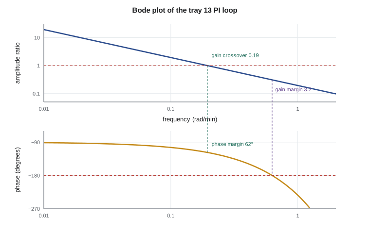
Gain and phase margins
Stability alone is not enough; a loop on the edge of stability is useless. Two margins measure how far a loop is from the edge. The gain margin is the factor by which the loop gain could rise before instability: the inverse of the open-loop amplitude ratio at the phase crossover. The phase margin is the extra phase lag that could be added at the gain crossover, where the amplitude ratio is 1, before the phase reaches \(-180°\). Common targets are a gain margin of 2 or more and a phase margin of 30° to 60°, the larger figures for loops whose models are uncertain.
With the SIMC tuning of lesson 8, \(K_c = 1.4\) %/°C and \(T_i = 6.5\) min, the tray 13 loop has a gain margin of 3.2 and a phase margin of 62°. The gain crossover is at 0.19 rad/min, which corresponds to a closed-loop response time of roughly \(1/0.19 \approx 5\) min. These are comfortable margins. To see why margins matter, the code doubles the dead time to 5 minutes, which might happen if the temperature measurement were moved two trays further away, or if the column ran at half rate. The gain margin falls to 1.6 and the phase margin to 34°. The loop would still be stable, but noticeably oscillatory, and a further increase in dead time or gain would push it over the edge.
| Frequency (rad/min) | Amplitude ratio with PI | Phase (degrees) |
|---|---|---|
| 0.03 | 6.46 | -94 |
| 0.10 | 1.94 | -104 |
| 0.20 | 0.97 | -119 |
| 0.30 | 0.65 | -133 |
| 0.50 | 0.39 | -162 |
Margins across the operating range
Margins are most useful as budgets. A gain margin of 3.2 means the product of every gain around the loop could rise by a factor of 3.2 before the loop became unstable; a phase margin of 62° means 62° of extra lag at the crossover frequency would do the same. Theo lists what could eat into those budgets on the recovery column. At half throughput the tray temperatures become more sensitive, so the process gain might rise by half. A fouled reboiler responds more slowly. A different feed composition moves the column profile, changing which trays are sensitive. A slower thermowell adds lag. Each change spends some of the margin, and several can happen together on a bad day.
Worked problem
Spending the gain margin
The tray 13 loop has a gain margin of 3.24 at design. At reduced rate the process gain rises by 50 %, and a worn steam valve raises the installed gain by a further 20 %. What gain margin remains?
Show solution
- Total gain increase: \(1.5 \times 1.2 = 1.8\).
- Remaining margin: \(3.24/1.8 = 1.8\).
Answer: About 1.8: still stable, but more oscillatory than at design. Combined with a longer dead time at low rate, the loop could approach the limit, which is why tuning is checked at the worst condition.
Nyquist and the robustness view
The Nyquist plot draws the open-loop response \(G_{OL}(j\omega)\) as a curve in the complex plane as \(\omega\) runs from zero to infinity. The point \(-1\) is critical: for an open-loop-stable process, the closed loop is stable if the curve does not encircle it. The shortest distance from the curve to \(-1\) is a single, very useful robustness measure, whose inverse is the maximum sensitivity \(M_s\), the largest value of \(|1/(1 + G_{OL})|\). A loop with \(M_s = 1.6\) can tolerate a substantial change in process gain or dead time; a loop with \(M_s = 3\) is close to the edge and will amplify disturbances in a band of frequencies. Lesson 8 reports \(M_s\) for each tuning rule.
What stability analysis teaches
Three lessons carry over to every chemical process loop. First, dead time sets a speed limit. No feedback controller can bring a loop to its set point faster than roughly the dead time, and trying to do so with high gain destroys the margins. Second, loops change. Throughput, fouling, catalyst age and valve wear change gains and dead times, so a loop tuned with thin margins at one condition will cycle at another. Third, the margins, not the speed, are what keep a loop in automatic. Operators trust loops that behave the same way every day.
Theo prepares a one-page note for Carla explaining the old oscillation: a gain at three-quarters of the ultimate gain, plus integral action, put the loop within a few percent of instability, so it rang at its ultimate period after every upset. The new tuning roughly triples the gain margin. He suggests one more change, which Malik approves: the tray 13 thermowell will be replaced by a fast-response design during the next shutdown, cutting the measurement lag by about half a minute and giving the loop a little more room.
Common mistakes
MistakeApplying the Routh test to a loop with dead time.
InsteadRouth needs polynomials; use frequency response or a Padé approximation.
MistakeJudging a loop only by whether it is stable.
InsteadCheck gain and phase margins or the maximum sensitivity.
MistakeAssuming more gain always gives faster, better control.
InsteadBeyond a point it only erodes the margins; dead time sets the speed limit.
MistakeTuning at one throughput and forgetting the dead time changes with rate.
InsteadCheck the margins at the slowest expected condition.
Summary and key terms
- A loop is stable if all roots of \(1 + G_{OL} = 0\) have negative real parts; Routh tests polynomials directly.
- The hold-tank loop has \(K_u = 77.5\) kW/K and \(P_u = 25\) min.
- Dead time adds unlimited phase lag; tray 13 has \(K_u = 5.27\) %/°C and \(P_u = 8.8\) min.
- With \(K_c = 1.4\), \(T_i = 6.5\) min the loop has a gain margin of 3.2 and a phase margin of 62°.
- Doubling the dead time halves the gain margin; margins must cover the worst operating condition.
- Characteristic equation
- The equation 1 + G_OL(s) = 0 whose roots are the closed-loop poles.
- Ultimate gain
- The proportional gain at which a loop oscillates with constant amplitude.
- Ultimate period
- The period of oscillation at the ultimate gain.
- Phase crossover
- The frequency at which the open-loop phase reaches minus 180 degrees.
- Gain margin
- The factor by which loop gain could increase before instability.
- Phase margin
- The extra phase lag at gain crossover that would make the loop unstable.
- Maximum sensitivity
- The peak of the magnitude of 1/(1 + G_OL); its inverse is the closest approach to minus one.
Practice problems
Work each problem on paper first, then reveal the answer to check.
A cubic characteristic polynomial has \(a_3 = 10\), \(a_2 = 12\), \(a_1 = 5\). What is the largest stable \(a_0\)?
Show answer
\(12 \times 5/10 = 6\).
At the phase crossover a loop's amplitude ratio is 0.4. What is its gain margin?
Show answer
2.5.
An FOPDT process has \(\theta = 1\) and \(\tau = 1\) min. What phase lag does the dead time add at 1 rad/min?
Show answer
1 radian, about 57°.
How many first-order lags, with no dead time, are needed before proportional control alone can make a loop unstable?
Show answer
Three: each lag adds at most 90° of phase lag.
The loop's phase margin is 15°. What will its set-point response look like?
Show answer
Strongly oscillatory, with large overshoot.
Name two plant changes that raise a loop's dead time.
Show answer
Lower throughput, or moving the sensor further from the manipulated variable.
Lesson quiz · 5 questions
Score 60% or more to complete this lesson.
Create a free account to save your progress, take quizzes and earn a certificate.