How machines learn from data

Machine learning sounds mysterious, but its core idea is simple: instead of writing the rules yourself, you choose a flexible model with adjustable numbers (parameters), define a way to measure how wrong it is on examples, and let an algorithm adjust the parameters to make it less wrong. Almost every modern AI system, from a spam filter to a large language model, works this way at heart. The differences lie in the kind of model, the amount of data and the scale of the computation.

This chapter builds that idea from the ground up with small, runnable Python programs. You will fit a model by gradient descent, see why a model that is perfect on its training data can still be useless, classify new cases from the nearest examples, train an artificial neuron, and measure whether a classifier is any good. You need only Python and NumPy (ENCM-100 or CMPUT-174 covers the basics); later courses (CMPUT-367, AI-210 and AI-310) develop the mathematics properly.

Data, features and labels

Machine learning starts with a dataset: a collection of examples. Each example is described by features, the measured inputs, such as outdoor temperature, vibration level or the pixels of an image. In supervised learning, each example also has a label: the answer we want the model to predict, such as cooling power, "failed" or "healthy", or "cat".

• Regression predicts a number: tomorrow's electricity demand, a building's energy use, the strength of a concrete mix.
• Classification predicts a category: spam or not spam, which of 1000 objects is in an image, whether a pump will fail this month.

Two other broad kinds of learning complete the picture:

• Unsupervised learning finds structure in data without labels: grouping similar customers (clustering), compressing data, or spotting unusual readings (anomaly detection).
• Reinforcement learning learns by trial and error from rewards: an agent takes actions in an environment and gradually learns which actions lead to high reward. It powered AlphaGo and is used to fine-tune language models (Lesson 4; AI-330).

A large language model is first trained with a form of self-supervised learning: the "label" for each position in a text is simply the next word, so the labels come free with the data. That is how such models can learn from trillions of words that nobody labelled by hand.

Learning as minimizing error

Suppose a data centre operator wants to predict the cooling power a data hall needs from the outdoor temperature. A simple model is a straight line:

where \(T\) is the temperature, \(\hat{P}\) the predicted power, and \(w\) and \(b\) are parameters to learn. To say how good a choice of \(w\) and \(b\) is, define a loss function. The usual choice for regression is the mean squared error over the \(n\) training examples:

Learning means finding the \(w\) and \(b\) that make \(L\) as small as possible. For a straight line there is a formula (least squares, from STAT-235), but for the huge models of modern AI there is no formula, so we use the method that works for all of them: gradient descent.

Gradient descent

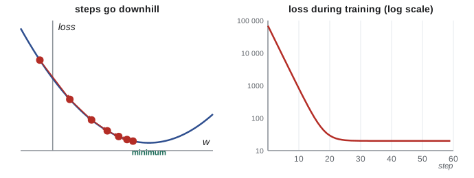
Picture the loss as a landscape over the parameters. The gradient points uphill, in the direction of steepest increase. Gradient descent takes repeated small steps the other way:

The step size \(\eta\) is the learning rate. Too small and learning is slow; too large and the steps overshoot and the loss can blow up. For the squared-error loss, the derivatives are \(\partial L/\partial w = \frac{2}{n}\sum (\hat{P}_i - P_i)T_i\) and \(\partial L/\partial b = \frac{2}{n}\sum(\hat{P}_i - P_i)\).

import numpy as np

# Outdoor temperature (°C) and cooling power (kW) for one data hall
T = np.array([-20, -10, -5, 0, 5, 10, 15, 20, 25, 30])
P = np.array([105, 168, 180, 214, 236, 262, 297, 318, 352, 371])

# Scale the input so gradient descent behaves well
x = (T - T.mean()) / T.std()

w, b = 0.0, 0.0          # start knowing nothing
lr = 0.1                 # learning rate
for step in range(200):
    pred = w * x + b
    err = pred - P
    loss = np.mean(err ** 2)
    w -= lr * 2 * np.mean(err * x)    # gradient of the loss with respect to w
    b -= lr * 2 * np.mean(err)        # ... and with respect to b
    if step in (0, 10, 50, 199):
        print(f"step {step:3d}: loss = {loss:9.1f}")

slope = w / T.std()                   # kW per °C in original units
intercept = b - slope * T.mean()
print(f"P = {intercept:.1f} + {slope:.2f} T")
print(f"Prediction at 28 °C: {intercept + slope * 28:.0f} kW")

Output: step 0: loss = 69266.3; step 10: loss = 818.3; step 50: loss = 19.9; step 199: loss = 19.9; P = 212.9 + 5.34 T; Prediction at 28 °C: 363 kW.

The program starts with \(w = b = 0\), which predicts 0 kW for everything (a loss of about 69,000), and within 50 steps finds the best line: about 213 kW at 0 °C, rising 5.34 kW per degree. A least-squares formula gives the same answer, which is a useful check. Two practical details matter even in this tiny example: the temperatures were standardized (shifted to mean 0 and scaled to standard deviation 1) so that the steps are well balanced, and the remaining loss of about 20 kW² reflects scatter in the data that no straight line can remove.

Exactly the same loop, with a model of billions of parameters instead of two and derivatives computed automatically by backpropagation, trains today's neural networks.

Generalization: the point of learning

A model is useful only if it works on new data it has never seen. Memorizing the training examples is easy; generalizing from them is the real goal. The standard way to check is to split the data: train on one part and measure error on a held-out test set that the training process never touches.

A model can fail in two opposite ways:

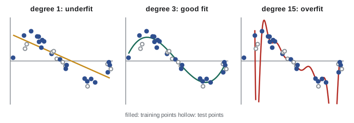
• Underfitting: the model is too simple to capture the pattern, so it does badly on both training and test data.
• Overfitting: the model is so flexible that it fits the noise in the training data, doing well on training data and badly on new data.

import numpy as np
import warnings
warnings.filterwarnings("ignore")      # high-degree fits trigger a conditioning warning

rng = np.random.default_rng(1)
x = np.sort(rng.uniform(0, 1, 30))
y = np.sin(2 * np.pi * x) + rng.normal(0, 0.2, 30)

idx = rng.permutation(30)
train, test = idx[:20], idx[20:]      # 20 examples to learn from, 10 held back

for degree in (1, 3, 9, 15):
    coef = np.polyfit(x[train], y[train], degree)
    mse_train = np.mean((np.polyval(coef, x[train]) - y[train]) ** 2)
    mse_test = np.mean((np.polyval(coef, x[test]) - y[test]) ** 2)
    print(f"degree {degree:2d}: train error {mse_train:.3f}   test error {mse_test:.3f}")

Output: degree 1: train error 0.222, test error 0.163; degree 3: train error 0.024, test error 0.050; degree 9: train error 0.012, test error 0.125; degree 15: train error 0.006, test error 2.298.

The data come from a sine wave plus noise. A straight line (degree 1) underfits: both errors are high. A cubic (degree 3) captures the pattern: low training error and the lowest test error. As the degree rises further, training error keeps falling toward zero, but test error rises; at degree 15 the curve wiggles wildly between the training points and its test error is about 46 times the cubic's. Lower training error is not the same as a better model.

Practitioners guard against overfitting by keeping a test set untouched until the end, using a third validation set (or cross-validation) to choose settings like the polynomial degree, collecting more data, and using regularization, which penalizes overly complex models. Deep learning adds its own techniques, but the principle is the same.

Learning from neighbours

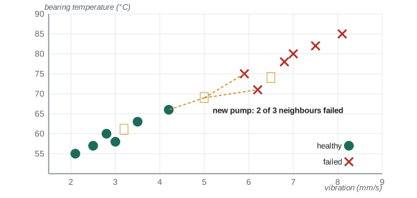
Not every learning method minimizes a loss with gradient descent. One of the simplest, k-nearest neighbours (k-NN), does no training at all: it stores the examples, and to classify a new case it finds the k most similar stored examples and takes a vote.

import numpy as np

# Each pump: [vibration (mm/s), bearing temperature (°C)], label 1 = failed within a month
X = np.array([[2.1, 55], [2.8, 60], [3.0, 58], [3.5, 63], [4.2, 66], [2.5, 57],
              [6.8, 78], [7.5, 82], [5.9, 75], [8.1, 85], [6.2, 71], [7.0, 80]])
y = np.array([0, 0, 0, 0, 0, 0, 1, 1, 1, 1, 1, 1])

# Put both features on a similar scale
mu, sd = X.mean(axis=0), X.std(axis=0)
Z = (X - mu) / sd

def predict(new, k=3):
    z = (np.array(new) - mu) / sd
    dist = np.sqrt(((Z - z) ** 2).sum(axis=1))
    nearest = np.argsort(dist)[:k]
    return int(round(y[nearest].mean())), y[nearest]

for pump in ([3.2, 61], [6.5, 74], [5.0, 69]):
    label, votes = predict(pump)
    print(pump, "-> votes", votes, "-> predict", "FAIL" if label else "ok")

Output: [3.2, 61] -> votes [0 0 0] -> predict ok; [6.5, 74] -> votes [1 1 1] -> predict FAIL; [5.0, 69] -> votes [0 1 1] -> predict FAIL.

The first two pumps are clearly like the healthy and failed groups. The third sits between them and is classified by a 2-to-1 vote, so the prediction is less certain. Notice the scaling step: without it, temperature (values around 70) would dominate distance over vibration (values around 5) simply because of its units. Choosing and preparing features well is often more important than the choice of algorithm.

Artificial neurons and neural networks

An artificial neuron computes a weighted sum of its inputs, adds a bias, and passes the result through an activation function:

Rosenblatt's perceptron (1958) used a step function: output 1 if the sum is positive, otherwise 0. It learns with a simple rule: whenever it gets an example wrong, nudge the weights toward the correct answer.

import numpy as np

# Learn the logical AND of two inputs with a single artificial neuron
X = np.array([[0, 0], [0, 1], [1, 0], [1, 1]])
y = np.array([0, 0, 0, 1])

w = np.zeros(2)
b = 0.0
for epoch in range(10):
    mistakes = 0
    for xi, target in zip(X, y):
        out = 1 if xi @ w + b > 0 else 0
        if out != target:                  # perceptron rule: nudge toward the right answer
            w += (target - out) * xi
            b += (target - out)
            mistakes += 1
    print(f"epoch {epoch}: mistakes {mistakes}, w = {w}, b = {b}")
    if mistakes == 0:
        break

Output: epoch 0: mistakes 1, w = [1. 1.], b = 1.0; epoch 1: mistakes 3, w = [2. 1.], b = 0.0; epoch 2: mistakes 3, w = [2. 1.], b = -1.0; epoch 3: mistakes 2, w = [2. 2.], b = -1.0; epoch 4: mistakes 1, w = [2. 1.], b = -2.0; epoch 5: mistakes 0, w = [2. 1.], b = -2.0.

A single neuron can only separate classes with a straight line (a flat plane in higher dimensions). That is why it cannot learn XOR, whose true and false cases cannot be separated by one line, the limitation Minsky and Papert identified in 1969. The fix is to stack neurons in layers: a neural network. Each layer's outputs feed the next, and with smooth activation functions (such as the rectified linear unit, ReLU, which outputs \(\max(0, z)\)) the whole network can be trained by gradient descent, with backpropagation computing all the derivatives efficiently.

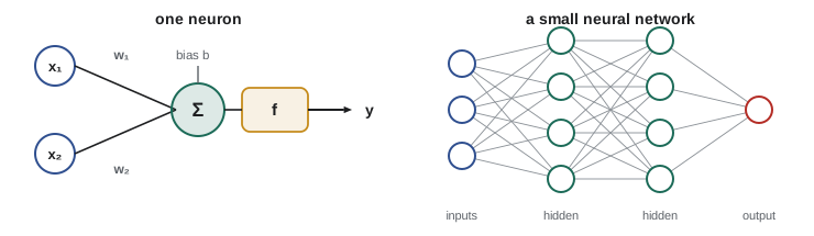
With enough neurons, networks can approximate almost any function. "Deep" networks with many layers learn useful features automatically: in an image network, early layers respond to edges and textures, middle layers to parts of objects, later layers to whole objects. Nobody programs these features; they emerge from minimizing the loss on millions of examples. That is the source of deep learning's power, and also why its internal workings are hard to interpret (AI-430).

Is the classifier any good?

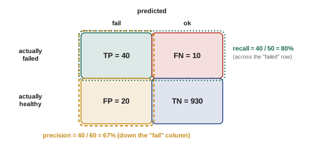
Accuracy, the fraction of predictions that are correct, is the obvious measure, but it can mislead badly when one class is rare. A confusion matrix shows all four outcomes for a two-class problem: true positives (TP), false positives (FP), false negatives (FN) and true negatives (TN). Two more measures come from it:

• Precision = TP / (TP + FP): of the cases the model flagged, how many were real?
• Recall = TP / (TP + FN): of the real cases, how many did the model catch?

Choosing which errors matter more is not a technical question alone. For a cancer screening test, missing a case (low recall) can be fatal; for a spam filter, blocking a real email (low precision) may be worse than letting spam through. Engineers set the trade-off with the people affected, and Lesson 5 shows that the same choices raise questions of fairness.

The recipe, in summary

Every machine learning project follows roughly the same steps: define the task and how success will be measured; collect and clean data; split it into training, validation and test sets; choose features and a model; train by minimizing a loss; tune settings on the validation set; evaluate once on the test set; then deploy and keep monitoring, because the world changes and a model's accuracy can drift (AI-420). Most of the effort in real projects goes into data and evaluation, not the learning algorithm.