
ROB-360 · Lesson 5 of 12 · 29 min
Simulation fundamentals: physics engines, time steps and real-time factor
Simulation lets a robot team drive a thousand routes overnight, crash into walls without cost, test behavior in rain that never comes to the test site and run the same scenario again and again until a bug is understood. It is also easy to misuse: a simulation that looks convincing can be wrong in ways that matter, and a team that trusts it blindly ships software tuned to a world that does not exist. This lesson explains what a robot simulator actually computes, how numerical integration, time steps and contacts shape the results, what the real-time factor means, and how the main simulators compare. Lesson 6 covers building models and worlds, and lesson 8 covers closing the gap between simulation and reality.
What a robot simulator does
A robot simulator combines several models. A physics engine advances the state of rigid bodies (positions, orientations, velocities) under forces, joint constraints and contacts. Sensor models generate what cameras, lidars, IMUs, encoders and GPS receivers would report, usually with added noise. Actuator models turn commands into forces or velocities, sometimes including motor limits and delays. A rendering engine draws images for cameras and for people watching. An interface layer connects all of this to the robot software, in ROS 2 typically through bridge nodes that publish simulated sensor topics and subscribe to commands, together with a simulated clock.
The physics engine is the core. At each time step it gathers the forces on every body, detects which bodies are touching, computes the contact and constraint forces that prevent interpenetration and keep joints together, and integrates the equations of motion forward by one step. Rigid-body dynamics follows the same Newton–Euler equations met in ROB-300; the difficulty lies in contacts and in doing it fast and stably for many bodies.
Numerical integration and stability
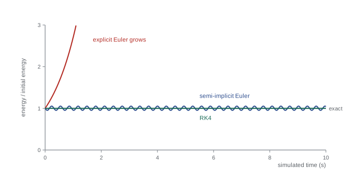
Simulators advance the state by discrete time steps h, replacing the continuous equations with an update rule. The simplest is explicit (forward) Euler: new position from old velocity, new velocity from old acceleration. It is cheap but unstable for stiff or oscillating systems: for an undamped spring it steadily adds energy until the motion explodes. Semi-implicit (symplectic) Euler updates velocity first and then uses the new velocity to update position. It costs the same but keeps energy bounded for oscillators, which is why many physics engines use it. Higher-order methods such as fourth-order Runge–Kutta (RK4) are more accurate per step but cost several force evaluations per step and do not mix easily with contact constraints.
import math
# Undamped mass-spring: m x'' = -k x, m = 1 kg, k = 100 N/m (natural frequency 10 rad/s)
k, m, x0 = 100.0, 1.0, 0.1
E0 = 0.5 * k * x0**2
def energy(x, v): return 0.5 * m * v**2 + 0.5 * k * x**2
def explicit(x, v, h): return x + h * v, v - h * k / m * x
def semi(x, v, h):
    v = v - h * k / m * x
    return x + h * v, v
def rk4(x, v, h):
    f = lambda x, v: (v, -k / m * x)
    a1 = f(x, v); a2 = f(x + h/2*a1[0], v + h/2*a1[1])
    a3 = f(x + h/2*a2[0], v + h/2*a2[1]); a4 = f(x + h*a3[0], v + h*a3[1])
    return (x + h/6*(a1[0] + 2*a2[0] + 2*a3[0] + a4[0]),
            v + h/6*(a1[1] + 2*a2[1] + 2*a3[1] + a4[1]))
for h in (0.001, 0.01, 0.05):
    row = []
    for name, step in (("explicit", explicit), ("semi-implicit", semi), ("RK4", rk4)):
        x, v = x0, 0.0
        for _ in range(int(10 / h)):          # simulate 10 s
            x, v = step(x, v, h)
        row.append(f"{name} {energy(x, v) / E0:9.4g}")
print(f"h={h:5.3f} s energy ratio after 10 s: " + " ".join(row))h=0.001 s energy ratio after 10 s: explicit 2.718 semi-implicit 1.004 RK4 1 h=0.010 s energy ratio after 10 s: explicit 2.096e+04 semi-implicit 1.043 RK4 1 h=0.050 s energy ratio after 10 s: explicit 2.41e+19 semi-implicit 0.8074 RK4 0.9588
The output shows the pattern clearly. Explicit Euler gains energy at every step size and explodes at the larger ones; semi-implicit Euler keeps the energy bounded, oscillating around its true value rather than drifting away; RK4 is extremely accurate at small steps but starts to lose energy as the step grows. A useful rule for explicit schemes is that the step must be small compared with the fastest natural period in the system. Stiff contacts and stiff joint controllers create very fast dynamics, which is why physics engines use implicit or semi-implicit formulations and why simulations can blow up when a gain is raised or a contact is made very stiff.
Worked problem
Choosing a time step
A robot arm joint behaves like a mass-spring with stiffness 4000 N·m/rad (from its controller and gearbox) and inertia 0.4 kg·m². Estimate its natural frequency and a reasonable maximum step if we want at least 20 steps per period.
Show solution
- Natural frequency: \( \omega_n = \sqrt{k/J} = \sqrt{4000/0.4} = 100 \) rad/s.
- Period: \( T = 2\pi/\omega_n \approx 0.063 \) s.
- At 20 steps per period: \( h \le 0.063/20 \approx 3.1 \) ms.
Answer: About 3 ms, so the default 1 ms step used by many simulators is comfortable. Doubling the controller stiffness would raise the frequency by \( \sqrt{2} \) and shrink the safe step accordingly.
Contacts and friction
Contacts are the hardest part of robot simulation. Real contacts are stiff, short-lived and governed by friction that switches between sticking and sliding. Physics engines model them in two broad ways. Penalty methods treat contact as a very stiff spring and damper that pushes bodies apart in proportion to how far they interpenetrate; they are simple but need small steps and allow some penetration. Constraint-based methods formulate contact as a complementarity problem: contact forces must be non-negative, bodies must not penetrate, and forces exist only where bodies touch. These are solved at each step, often approximately and iteratively, with parameters such as the number of solver iterations and error-reduction terms that affect accuracy and stability.
Friction is usually modeled with Coulomb's law, the friction force limited to μ times the normal force, approximated by a pyramid in many solvers. Wheels, grippers and feet depend critically on friction, and simulated grasps or wheel slip can differ greatly from reality if μ, contact stiffness or the contact geometry are wrong. A common symptom is jitter: objects that should rest quietly vibrate or creep because the solver never quite converges. Remedies include smaller steps, more solver iterations, softer contact parameters, better mass ratios between touching bodies and simpler collision shapes.
Worked problem
Can the wheel push the cart?
A simulated mobile base of 40 kg must push a 25 kg cart with rolling resistance coefficient 0.05. Its drive wheels carry the whole robot weight, with simulated friction coefficient μ = 0.6. Will the wheels slip, and what happens if a modeler sets μ = 0.05 by mistake?
Show solution
- Force needed: \( 0.05 \times 25 \times 9.81 \approx 12.3 \) N plus the robot's own rolling resistance \( 0.05 \times 40 \times 9.81 \approx 19.6 \) N: about 32 N.
- Available traction at μ = 0.6: \( 0.6 \times 40 \times 9.81 \approx 235 \) N, ample.
- At μ = 0.05: \( 0.05 \times 392 \approx 19.6 \) N, less than 32 N, so the wheels spin.
Answer: With μ = 0.6 the push works; with a mistyped μ = 0.05 the simulated wheels spin and the test fails for a reason that has nothing to do with the software. Friction parameters deserve review like code.
Simulated time and the real-time factor
A simulator keeps its own clock. Each physics step advances simulated time by h; how long that takes in wall-clock time depends on the computer and the scene. The real-time factor (RTF) is the ratio of simulated time to wall-clock time: an RTF of 1.0 means the simulation keeps pace with reality, 0.5 means it runs at half speed and 5.0 means five times faster. Robot software in simulation must use the simulated clock (use_sim_time in ROS 2, with the simulator publishing on the /clock topic); otherwise timeouts, controllers and filters behave wrongly whenever the RTF is not exactly 1.
Running faster than real time is valuable for testing: a 30-minute mission at an RTF of 6 takes 5 minutes. But the robot software must then compute six times faster too, or it will appear to the simulated world as if it were slow. Many test setups therefore run in lock-step, where the simulator waits for the software to finish each control cycle, which gives deterministic results at the cost of speed.
Worked problem
Planning a nightly simulation run
A regression suite has 400 simulated missions averaging 6 minutes of simulated time each. The simulator achieves an RTF of 3 on one CI machine. How long does the suite take on one machine and on 8 machines in parallel?
Show solution
- Total simulated time: \( 400 \times 6 = 2400 \) min.
- Wall-clock time at RTF 3: \( 2400 / 3 = 800 \) min, about 13.3 h on one machine.
- On 8 machines: \( 800 / 8 = 100 \) min, about 1.7 h, plus start-up overhead.
Answer: About 13 h on one machine or under 2 h on eight. Real-time factor, parallelism and scenario length together decide whether a suite fits in a nightly window.
Determinism
A simulation is deterministic if the same inputs always produce exactly the same outputs. Determinism is precious for debugging and for regression tests, but it is easy to lose: multithreaded physics solvers, random sensor noise without fixed seeds, rendering on GPUs, robot software that runs asynchronously with the simulator and messages that arrive in different orders all introduce variation. Teams aim for determinism in unit-level and short integration tests (fixed seeds, lock-step stepping, single-threaded physics) and accept controlled variation in larger scenario tests, judging those by statistics over many runs rather than by one exact trace.
The simulators in use
Several simulators are common in robotics at the time of writing. Gazebo (formerly Ignition) is the open-source simulator most closely tied to ROS: its LTS releases are paired with ROS 2 LTS distributions, Harmonic with Jazzy and Jetty, released in September 2025, with Lyrical, and the ros_gz packages bridge topics and the clock. It uses pluggable physics engines (DART by default, with others available) and supports many sensors. NVIDIA Isaac Sim, built on the Omniverse platform, offers photorealistic GPU rendering and GPU-accelerated physics and is popular for perception and learning work. MuJoCo, developed for contact-rich control and open-sourced by DeepMind in 2022, is fast and accurate for articulated bodies and widely used in reinforcement learning. Webots, open source since 2018, is easy to start with and common in education. Commercial and domain-specific tools cover autonomous driving, drones and industrial cells.
| Simulator | Strengths | Typical use |
|---|---|---|
| Gazebo (Harmonic, Jetty) | Tight ROS 2 integration, open source, many sensors and plugins | Navigation and integration testing |
| NVIDIA Isaac Sim | Photorealistic rendering, GPU physics, synthetic data tools | Perception, manipulation, learning |
| MuJoCo | Fast, accurate contact dynamics for articulated systems | Control research, reinforcement learning |
| Webots | Easy setup, large robot library | Teaching and prototyping |
| Domain-specific tools | Detailed vehicle, traffic or aerial models | Driving and drone testing |
Choosing a simulator is an architectural decision worth an ADR (lesson 2). The right choice depends on what must be trusted: wheel and navigation behavior, camera realism, contact-rich manipulation or the speed to run millions of episodes. Many teams use more than one, for example Gazebo for nightly integration tests of the full ROS 2 stack and a GPU simulator for training perception models.
Common mistakes
MistakeRaising a simulated controller gain until the simulation explodes and blaming the simulator
InsteadCheck the step size against the system's fastest dynamics; stiff systems need smaller steps.
MistakeRunning robot nodes on wall-clock time in simulation
InsteadSet use_sim_time so nodes follow the simulator's /clock.
MistakeAssuming a grasp that works in simulation will work in reality
InsteadContact and friction parameters dominate grasps; validate them against real tests.
MistakeComparing one simulated run against one real run
InsteadJudge stochastic scenarios with statistics over many runs.
MistakePicking a simulator because it looks realistic
InsteadChoose for the physics, sensors and speed your tests need, and record the decision.
Summary and key terms
- A robot simulator combines physics, sensor, actuator and rendering models with an interface to the robot software and a simulated clock.
- Numerical integration replaces continuous dynamics with discrete steps; explicit Euler gains energy, semi-implicit Euler stays bounded and RK4 is accurate but costly.
- Time steps must be small compared with the fastest dynamics, which stiff controllers and contacts make very fast.
- Contacts and friction are modeled with penalty or constraint methods and are the main source of simulation error and jitter.
- The real-time factor is simulated time over wall-clock time; robot software must follow the simulated clock.
- Determinism helps debugging; larger scenario tests are judged statistically.
- Gazebo, Isaac Sim, MuJoCo and Webots have different strengths, so the choice should follow what the tests must trust.
- Physics engine
- Software that advances rigid-body states under forces, constraints and contacts.
- Time step
- The interval of simulated time advanced by one update.
- Explicit Euler
- An integrator that updates position and velocity from the old state only.
- Semi-implicit Euler
- An integrator that updates velocity first and uses it to update position, keeping oscillator energy bounded.
- RK4
- The fourth-order Runge–Kutta method, accurate but needing four evaluations per step.
- Penalty contact
- A contact model using stiff springs that resist interpenetration.
- Complementarity
- The condition that contact force and gap cannot both be non-zero.
- Real-time factor
- The ratio of simulated time to wall-clock time.
- Lock-step simulation
- Stepping the simulator only when the robot software has finished each cycle.
- Determinism
- The property that identical inputs always give identical outputs.
Practice problems
Work each problem on paper first, then reveal the answer to check.
Which integrator in the listing gained energy at every step size?
Show answer
Explicit Euler.
Why do many physics engines use semi-implicit Euler?
Show answer
It costs the same as explicit Euler but keeps oscillator energy bounded.
A joint has natural frequency 200 rad/s. What step gives 20 steps per period?
Show answer
About 1.6 ms.
Name the two broad approaches to contact modeling.
Show answer
Penalty methods and constraint-based (complementarity) methods.
What is a common symptom of poorly converged contacts?
Show answer
Jitter or creeping of objects that should be at rest.
What does an RTF of 0.5 mean?
Show answer
The simulation runs at half real-time speed.
Which topic carries simulated time in ROS 2?
Show answer
/clock.
How long does 600 min of simulated time take at RTF 4?
Show answer
150 min.
Name two sources of nondeterminism in simulation.
Show answer
For example multithreaded solvers and unseeded random noise.
Which Gazebo LTS release pairs with ROS 2 Lyrical?
Show answer
Jetty.
Lesson quiz · 5 questions
Score 60% or more to complete this lesson.
Create a free account to save your progress, take quizzes and earn a certificate.