
ROB-230 · Lesson 3 of 12 · 29 min
Convolution and the impulse response
Lesson 2 claimed that a linear time-invariant system is completely described by one function, its impulse response. This lesson proves that claim and turns it into a calculation. The idea is simple and beautiful: any input can be written as a sum of shifted, scaled impulses; by linearity and time invariance, the output is the same sum of shifted, scaled impulse responses. The operation that performs this sum is called convolution. Convolution is how a sensor's dynamics blur a measurement, how a moving-average filter smooths encoder data, how a motor's inertia turns a torque pulse into a lingering velocity, and how a camera's lens blurs an image. It also explains why the Laplace and Fourier transforms of later lessons are so useful: they turn convolution into multiplication.
The impulse response
The impulse response h(t) of an LTI system is its output when the input is a unit impulse \( \delta(t) \) and the system starts at rest. In discrete time, h[n] is the output sequence produced by the input \( \delta[n] \), which is 1 at n = 0 and 0 elsewhere. The impulse response is a fingerprint. A first-order low-pass sensor has \( h(t) = \frac{1}{\tau}e^{-t/\tau}u(t) \), an instant jump that decays with time constant \( \tau \). A three-sample moving average has \( h[n] = \tfrac{1}{3} \) for n = 0, 1, 2 and zero otherwise. A lightly damped robot link struck by a hammer rings with a decaying oscillation, and that ringing is its impulse response; structural engineers measure it with an instrumented hammer and an accelerometer to identify vibration modes.
The impulse response also answers the questions of lesson 2 at a glance. The system is causal if h(t) = 0 for t < 0: it cannot respond before the impulse arrives. It is memoryless only if h is itself an impulse. And it is BIBO-stable exactly when the impulse response is absolutely integrable:
The decaying exponential passes this test; an integrator, whose impulse response is the unit step, fails it, consistent with lesson 2.
Building the convolution sum
Start in discrete time, where everything is a finite sum. Any input sequence can be written as a sum of scaled, shifted impulses, one per sample:
This just says the signal at n is its value at n. Now apply the system. Time invariance says the response to \( \delta[n - k] \) is \( h[n - k] \); linearity says the response to the weighted sum is the weighted sum of responses. So
This is the convolution sum, written with an asterisk. In words: each past input sample x[k] launches its own copy of the impulse response, starting at time k and scaled by x[k], and the output at time n is the sum of all those copies that are still ringing. For a causal system and an input that starts at n = 0, the sum runs only from k = 0 to k = n. The continuous-time version follows the same reasoning with integrals:
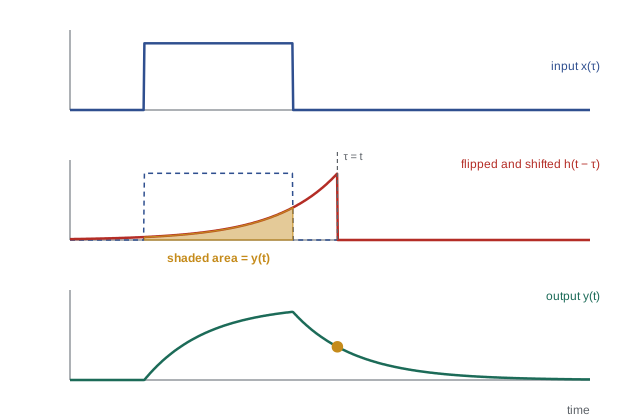
Flip, slide, multiply, add
Computing a convolution by hand follows a mechanical recipe. Write the input as a function of the dummy variable \( \tau \). Flip the impulse response to get \( h(-\tau) \), then slide it by t to get \( h(t - \tau) \). Multiply the two functions point by point, and integrate (or sum) the product. Repeat for every t of interest. As t increases, the flipped impulse response slides from left to right across the input, and the output traces the changing area of overlap. The flipping is what puts the most recent inputs at the front of the impulse response, where its weight is greatest for a typical decaying system: a sensor remembers recent inputs strongly and old ones faintly.
Convolution has useful algebraic properties. It is commutative (\( x * h = h * x \)), so either function can be flipped. It is associative, so two systems in series with impulse responses \( h_1 \) and \( h_2 \) act as one system with \( h_1 * h_2 \), and the order of LTI blocks in a cascade does not matter. It distributes over addition, so parallel systems add their impulse responses. And convolving with \( \delta(t - t_0) \) simply delays a signal by \( t_0 \), which is how a pure transport delay appears in this framework.
Worked problem
A moving average by convolution
Encoder velocity estimates (rad/s) arrive as x = [0, 0, 3, 3, 3, 9, 3, 3] for n = 0 to 7; the 9 is a glitch. Apply the causal three-point average \( h[n] = \tfrac{1}{3} \) for n = 0, 1, 2. Find y[n].
Show solution
- \( y[n] = \tfrac{1}{3}(x[n] + x[n-1] + x[n-2]) \), taking x = 0 before n = 0.
- y[0] = 0, y[1] = 0, y[2] = 1, y[3] = 2, y[4] = 3.
- y[5] = (9 + 3 + 3)/3 = 5, y[6] = (3 + 9 + 3)/3 = 5, y[7] = (3 + 3 + 9)/3 = 5.
Answer: y = [0, 0, 1, 2, 3, 5, 5, 5]. The filter turns the step into a ramp lasting two samples, a delay of about one sample, and it spreads the glitch over three samples at one-third height rather than removing it. A median filter would remove it; averaging cannot, which is why outliers need separate treatment.
Worked problem
Step response of a first-order sensor by convolution
A temperature sensor has impulse response \( h(t) = \frac{1}{\tau}e^{-t/\tau}u(t) \) with \( \tau = 4 \) s. Find its response to a unit step, and the reading 8 s after the true temperature jumps by 10 °C.
Show solution
- For t ≥ 0, \( y(t) = \int_0^t \frac{1}{\tau}e^{-(t-\sigma)/\tau}\,d\sigma \), since the step is 1 for every σ between 0 and t.
- \( = \frac{1}{\tau}e^{-t/\tau}\int_0^t e^{\sigma/\tau}\,d\sigma = e^{-t/\tau}\,(e^{t/\tau} - 1) = 1 - e^{-t/\tau} \).
- For a 10 °C step at t = 8 s: \( 10\,(1 - e^{-2}) = 10 \times 0.865 = 8.65 \) °C.
Answer: The step response is \( 1 - e^{-t/\tau} \), and after two time constants the sensor shows 8.65 °C of the 10 °C change. Readings taken too soon after a change are biased low, a direct consequence of the sensor convolving the truth with its impulse response.
Step response and impulse response are related
Because the step is the integral of the impulse, the step response s(t) of an LTI system is the integral of its impulse response, and the impulse response is the derivative of the step response:
This matters experimentally. True impulses are hard to apply without saturating or damaging something, but steps are easy: switch on a voltage, change a set point. Engineers therefore often measure the step response and differentiate it, although differentiation amplifies noise, so in practice parametric models are usually fitted to the step data instead (lesson 4). In discrete time the relations are a running sum and a first difference: \( s[n] = \sum_{k \le n} h[k] \) and \( h[n] = s[n] - s[n-1] \).
Convolution in robotics
Convolution appears wherever a system smooths, blurs or remembers.
- Sensor dynamics. Every sensor has an impulse response, so every measurement is the true signal convolved with it, plus noise. A slow force sensor smears a sharp impact; a gyroscope's internal filter delays fast rotations. Knowing h lets you predict, and sometimes partly undo, this distortion.
- Digital filters. A finite impulse response (FIR) filter, such as the moving average, is literally a convolution sum with a short, fixed list of coefficients. Lesson 11 designs them.
- Motion profiles. Convolving a velocity step with a short rectangular pulse produces a ramp; convolving twice gives an S-curve with limited jerk. Some motion controllers generate smooth trajectories exactly this way, by passing a crude command through cascaded moving-average filters.
- Images. Blurring, sharpening and edge detection on camera images are two-dimensional convolutions with small kernels, the basis of classical computer vision and of the convolutional neural networks used in ROB-330.
Worked problem
Shaping a motion profile with convolution
A conveyor robot's velocity command is a step to 0.5 m/s at t = 0. It is passed through a moving average of duration 0.2 s (impulse response height 5 s⁻¹ for 0 ≤ t < 0.2 s). Describe the resulting velocity and acceleration.
Show solution
- Convolving a step with a rectangle of unit area gives a linear ramp lasting the rectangle's duration.
- Velocity rises linearly from 0 to 0.5 m/s over 0.2 s and then holds.
- Acceleration is constant at \( 0.5/0.2 = 2.5 \) m/s² during the ramp and zero afterwards.
Answer: The filtered command reaches 0.5 m/s in 0.2 s with a bounded acceleration of 2.5 m/s², instead of the infinite acceleration of a raw step. Passing it through a second moving average would also bound the jerk, giving an S-curve.
Computing convolution
In software, a direct discrete convolution of an N-sample signal with an M-sample impulse response needs about N × M multiplications, which is cheap for short filters. NumPy's np.convolve does it in one call. For long impulse responses, the fast Fourier transform of lesson 8 computes the same result much faster, because convolution in time is multiplication in frequency. The code below applies a five-point moving average to a noisy step and confirms the delay and noise reduction predicted earlier in the course.
import numpy as np
rng = np.random.default_rng(7)
n = np.arange(400)
true = np.where(n >= 200, 1.0, 0.0)             # unit step at n = 200
x = true + rng.normal(0, 0.2, n.size)           # noisy measurement
h = np.ones(5) / 5                              # five-point moving average
y = np.convolve(x, h)[:n.size]                  # causal: keep first N outputs
sb, sa = np.std(x[:200]), np.std(y[5:200])
print("noise std before:", round(sb, 3), " after:", round(sa, 3))
print("reduction factor:", round(sb/sa, 2), " (theory sqrt(5) =", round(np.sqrt(5), 2), ")")
cross = np.argmax(np.convolve(true, h)[:n.size] >= 0.5)
print("filtered step crosses 0.5 at n =", cross, "(true step at n = 200)")noise std before: 0.174 after: 0.077 reduction factor: 2.27 (theory sqrt(5) = 2.24 ) filtered step crosses 0.5 at n = 202 (true step at n = 200)
The noise falls by roughly the square root of the filter length, and the filtered step reaches half height two samples late, at n = 202, half the filter length. That trade between noise reduction and delay is the central compromise of all filtering, and lesson 11 quantifies it precisely with group delay.
| Property | Statement | Consequence |
|---|---|---|
| Commutative | \( x * h = h * x \) | Either function may be flipped in a calculation |
| Associative | \( (x * h_1) * h_2 = x * (h_1 * h_2) \) | Cascaded LTI systems combine; order does not matter |
| Distributive | \( x * (h_1 + h_2) = x * h_1 + x * h_2 \) | Parallel systems add impulse responses |
| Identity | \( x * \delta = x \) | The impulse is the do-nothing system |
| Delay | \( x * \delta(t - t_0) = x(t - t_0) \) | Transport delay is convolution with a shifted impulse |
Common mistakes
MistakeForgetting to flip the impulse response
InsteadConvolution uses \( h(t - \tau) \); sliding an unflipped h computes correlation instead.
MistakeUsing np.convolve output at full length as a causal filter
InsteadThe full output has N + M − 1 samples; for a causal filter keep the first N.
MistakeExpecting a moving average to remove outliers
InsteadAveraging spreads a spike; use a median filter or validity checks for outliers.
MistakeDifferentiating a noisy measured step response to get h
InsteadDifferentiation amplifies noise; fit a model to the step response instead.
MistakeApplying convolution to a nonlinear or time-varying system
InsteadConvolution with a single h is valid only for LTI systems.
Summary and key terms
- The impulse response is the output of an LTI system to a unit impulse with zero initial conditions.
- Any input is a sum of shifted, scaled impulses, so the output is a sum of shifted, scaled impulse responses: the convolution sum or integral.
- Convolution is computed by flipping, sliding, multiplying and summing or integrating.
- A system is causal if h is zero for negative time and BIBO-stable if h is absolutely integrable or summable.
- The step response is the integral of the impulse response.
- Convolution is commutative, associative and distributive; cascaded LTI blocks combine by convolving their impulse responses.
- FIR filters, sensor dynamics, motion-profile shaping and image processing are all convolutions.
- Impulse response
- The output of an LTI system when the input is a unit impulse.
- Convolution
- The operation \( (x * h)(t) = \int x(\tau)h(t - \tau)\,d\tau \) that gives an LTI system's output.
- Convolution sum
- The discrete-time form \( \sum_k x[k]h[n - k] \).
- Step response
- The output of a system to a unit step; the integral of the impulse response.
- Absolutely integrable
- Having a finite integral of the absolute value; the stability condition on h.
- Moving average
- An FIR filter that averages the last N samples.
- FIR filter
- A filter whose impulse response has finite length.
- Kernel
- The short impulse response used in a convolution, especially for images.
- Transport delay
- A pure time shift, equivalent to convolution with a shifted impulse.
- Correlation
- A related operation that slides one signal over another without flipping.
Practice problems
Work each problem on paper first, then reveal the answer to check.
Convolve x = [1, 2, 3] with h = [1, 1].
Show answer
[1, 3, 5, 3].
What is the impulse response of y[n] = x[n − 3]?
Show answer
h[n] = δ[n − 3], a three-sample delay.
Two moving averages of length 3 are cascaded. What is the length of the combined impulse response?
Show answer
5 samples, a triangular shape [1, 2, 3, 2, 1]/9.
Is a system with \( h(t) = e^{t}u(t) \) stable?
Show answer
No; the integral of \( e^t \) diverges.
Find the step response of a system with \( h(t) = 2e^{-2t}u(t) \).
Show answer
\( 1 - e^{-2t} \) for t ≥ 0.
A moving average of length 10 runs at 1 kHz. Roughly how much delay does it add?
Show answer
About 4.5 samples, 4.5 ms.
By how much does a length-16 moving average reduce white-noise standard deviation?
Show answer
By a factor of 4.
Convolve a unit step with a rectangle of height 1 lasting 2 s.
Show answer
A ramp of slope 1 from t = 0 to 2, then constant at 2.
Why is the impulse response of a causal system zero for t < 0?
Show answer
The system cannot respond before the impulse is applied.
How many multiplications does direct convolution of 1,000 samples with a 50-tap filter need?
Show answer
About 50,000.
Lesson quiz · 5 questions
Score 60% or more to complete this lesson.
Create a free account to save your progress, take quizzes and earn a certificate.