
ROB-220 · Lesson 11 of 12 · 31 min
Calibration, filtering and sensor fusion basics
Raw sensor readings are never quite right. Earlier lessons showed that every sensor has biases, scale errors, misalignments, noise and drift, and that no single sensor covers every situation. This lesson brings those threads together into three practical skills. Calibration removes the systematic errors that can be measured and modeled. Filtering reduces random noise at the cost of delay. And sensor fusion combines sensors whose errors differ, so that each covers the other's weaknesses. The complementary filter developed here is the simplest useful fusion method and runs on countless drones and balancing robots; the Kalman filter, introduced briefly at the end, is developed properly in ROB-310.
Calibration: removing systematic error
Calibration compares a sensor's output with known references and fits a model that corrects it. The simplest model is linear, with an offset b and a scale factor s:
Two reference points determine both parameters; more points, fitted by least squares, average out noise and reveal nonlinearity. Multi-axis sensors need more. A three-axis accelerometer or magnetometer is modeled with a bias vector and a 3 × 3 matrix that captures scale factors, cross-axis coupling and misalignment. A classic procedure for accelerometers places the sensor in six orientations, each axis pointing up and then down, so that each axis sees +1 g and −1 g; the average of each pair gives the bias, and half the difference gives the scale. Magnetometers are calibrated by rotating the robot through as many orientations as possible: ideally the readings lie on a sphere, but hard-iron errors shift its center and soft-iron errors stretch it into an ellipsoid, and fitting the ellipsoid gives the correction.
Worked problem
Six-position accelerometer calibration
With its z-axis pointing straight up, an accelerometer reads 10.02 m/s² on z; pointing straight down, it reads −9.70 m/s². Find the z-axis bias and scale factor, and correct a later reading of 5.00 m/s².
Show solution
- Bias: \( b = (10.02 + (-9.70))/2 = 0.16 \) m/s².
- Scale: \( s = (10.02 - (-9.70))/(2 \times 9.81) = 19.72/19.62 = 1.0051 \).
- Corrected reading: \( (5.00 - 0.16)/1.0051 = 4.82 \) m/s².
Answer: A bias of 0.16 m/s² and a scale factor about 0.5 % high; the corrected reading is 4.82 m/s². Uncorrected, the bias alone is equivalent to nearly a degree of tilt error.
Calibration also covers the geometry between sensors, called extrinsic calibration: the exact transform from a camera, lidar or IMU to the robot's base frame (ROB-210). An error of one degree in a lidar's mounting angle places an obstacle 20 m away about 35 cm from where it really is. Camera-lidar, camera-IMU and hand-eye calibration procedures estimate these transforms from data, and the results are stored in the robot's transform tree. Calibration is never finished: temperature, vibration, wear and knocks change sensors over time, so robots need routine checks and often online calibration that estimates biases continuously during operation.
Filtering noise: moving averages and low-pass filters
Random noise cannot be calibrated away, but it can be reduced by filtering. A moving average of the last N samples cuts white noise by \( \sqrt{N} \), as lesson 1 showed, but it delays the signal by about \( (N-1)/2 \) samples. A more economical alternative is the first-order low-pass filter, also called an exponential moving average, which needs only the previous output:
The parameter \( \alpha \) between 0 and 1 sets the smoothing: values near 1 give heavy smoothing and slow response, values near 0 follow the raw signal. It corresponds to a time constant \( \tau \) and a cutoff frequency \( f_c = 1/(2\pi\tau) \). Every filter of this kind trades noise for lag, and lag in a feedback loop reduces stability margins (ROB-230 and ROB-300), so filters inside control loops must be chosen carefully. Outliers, such as a single wild lidar return or an encoder glitch, are better handled with a median filter or a validity check than with averaging, which smears them into neighboring samples.
Worked problem
Choosing a low-pass filter
A distance sensor is sampled at 50 Hz (\( \Delta t = 0.02 \) s). You want a cutoff of about 2 Hz. What \( \tau \) and \( \alpha \) should you use, and roughly how much delay does the filter add?
Show solution
- \( \tau = 1/(2\pi f_c) = 1/(2\pi \times 2) = 0.0796 \) s.
- \( \alpha = 0.0796/(0.0796 + 0.02) = 0.80 \).
- A first-order filter delays slowly varying signals by roughly \( \tau \), about 80 ms.
Answer: Use \( \alpha \approx 0.80 \), giving a 2 Hz cutoff and roughly 80 ms of delay. If 80 ms is too long for a fast robot, a faster but noisier filter, or fusion with another sensor, is needed.
Complementary sensors and the complementary filter
The real power of fusion comes from combining sensors whose errors live at different frequencies. Lesson 3 gave the classic example. A gyroscope measures rotation rate precisely and responds instantly, but its integrated angle drifts slowly: its errors are low-frequency. An accelerometer gives tilt from gravity with no drift, but is noisy and disturbed by every bump and acceleration: its errors are high-frequency. A complementary filter takes the high-frequency part of the gyroscope angle and the low-frequency part of the accelerometer angle and adds them, so each sensor contributes where it is good.
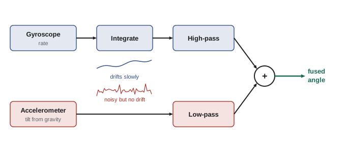
The weights sum to one, which is where the name comes from. The crossover time constant \( \tau = \alpha\Delta t/(1 - \alpha) \) decides which sensor dominates at which timescale: for changes faster than \( \tau \) the gyroscope wins, for slower changes the accelerometer corrects the drift. Typical values are \( \alpha = 0.98 \) at 100 Hz, giving a crossover of about half a second. The filter is a few lines of code, runs on the smallest microcontroller and works remarkably well, which is why it is found in self-balancing robots, gimbals and hobby drones.
Worked problem
Setting the complementary filter
An IMU is sampled at 200 Hz. You want the accelerometer to correct gyroscope drift over a time constant of about 1 s. What \( \alpha \) should you use? If the gyroscope has an uncorrected bias of 0.5 °/s, roughly what steady angle error remains?
Show solution
- \( \Delta t = 0.005 \) s. From \( \tau = \alpha\Delta t/(1 - \alpha) \): \( \alpha = \tau/(\tau + \Delta t) = 1/1.005 = 0.995 \).
- With a constant rate bias b, the filter settles where the accelerometer correction balances the drift: steady error \( \approx b\,\tau = 0.5 \times 1 = 0.5° \).
- Shorter \( \tau \) reduces this error but lets more accelerometer noise through.
Answer: Use \( \alpha \approx 0.995 \). An uncorrected 0.5 °/s bias leaves a steady error of about 0.5°, so it is still worth removing the gyroscope bias at start-up.
import numpy as np
rng = np.random.default_rng(3)
dt, n = 0.01, 3000                       # 100 Hz for 30 s
t = np.arange(n) * dt
true = 10 * np.sin(0.5 * t)              # true pitch, degrees
rate = np.gradient(true, dt)
gyro = rate + 0.8 + rng.normal(0, 0.3, n)              # 0.8 deg/s bias plus noise
acc = true + rng.normal(0, 3.0, n)                     # tilt from accelerometer, noisy
gyro_only = np.cumsum(gyro) * dt
alpha, est = 0.98, np.zeros(n)
for k in range(1, n):
    est[k] = alpha * (est[k-1] + gyro[k] * dt) + (1 - alpha) * acc[k]
def rms(e): return np.sqrt(np.mean(e**2))
print(f"accelerometer only : RMS error {rms(acc - true):5.2f} deg")
print(f"gyroscope only     : RMS error {rms(gyro_only - true):5.2f} deg (drifts)")
print(f"complementary 0.98 : RMS error {rms(est - true):5.2f} deg")accelerometer only : RMS error 3.01 deg gyroscope only : RMS error 14.03 deg (drifts) complementary 0.98 : RMS error 0.46 deg
The output shows the pattern clearly. Each sensor alone is poor, one noisy and one drifting, but the fused estimate is far better than either. This is the central idea of sensor fusion, and every more sophisticated method builds on it.
Toward the Kalman filter
The complementary filter uses a fixed blend. The Kalman filter, developed by Rudolf Kálmán in 1960 and used to navigate the Apollo spacecraft, generalizes the idea: it keeps an estimate of the state and of its uncertainty, predicts both forward with a motion model, and when a measurement arrives, blends prediction and measurement with a gain that depends on their relative uncertainties. A precise measurement gets a large weight; a noisy one a small weight. For a single quantity, the update looks like the complementary filter with a gain that adapts automatically:
Here \( P^{-} \) is the variance of the prediction and R the variance of the measurement noise, which is exactly what datasheet noise figures and the Allan analysis of lesson 3 provide. The extended and unscented Kalman filters, and particle filters, handle nonlinear robot models; they are the subject of ROB-310, and they underpin the localization and SLAM systems of ROB-340.
Worked problem
One Kalman update
A robot's predicted position along a corridor is 12.0 m with variance 0.25 m² (standard deviation 0.5 m). A UWB fix reports 12.6 m with variance 0.04 m² (standard deviation 0.2 m). Find the Kalman gain, the updated estimate and its variance \( (1 - K)P^{-} \).
Show solution
- \( K = 0.25/(0.25 + 0.04) = 0.862 \).
- Estimate: \( 12.0 + 0.862 \times (12.6 - 12.0) = 12.52 \) m.
- Variance: \( (1 - 0.862) \times 0.25 = 0.0345 \) m², a standard deviation of 0.19 m.
Answer: The estimate moves most of the way toward the more precise UWB fix, to 12.52 m, and the uncertainty shrinks below that of either source alone. Fusing two estimates always gives a result at least as good as the better one, if their noise levels are known correctly.
Time synchronization and practical fusion
Fusion only works if the measurements being combined refer to the same moment and the same frame. A camera image that is 60 ms old fused with a fresh IMU reading will place features in the wrong position whenever the robot moves. Good systems timestamp every measurement at acquisition, preferably in hardware, synchronize clocks between computers (for example with the Precision Time Protocol), trigger sensors together where possible and interpolate measurements to common times. In ROS 2, message headers carry timestamps and frame IDs for this reason, and tf2 interpolates transforms in time (ROB-110). Many baffling fusion bugs turn out to be a timestamp in the wrong clock, a missing extrinsic calibration or a frame mix-up rather than a problem with the filter.
| Problem | Symptom | Remedy |
|---|---|---|
| Unremoved bias | Steady offset or slow drift | Calibrate at start-up; estimate online |
| Wrong extrinsic calibration | Objects shift as the robot turns | Calibrate sensor-to-base transforms |
| Timestamp mismatch | Errors that grow with speed | Hardware timestamps; clock synchronization |
| Over-filtering | Sluggish, oscillating control | Less smoothing in the loop; fuse a faster sensor |
| Wrong noise values | Filter trusts the wrong sensor | Measure noise (Allan variance); tune carefully |
Common mistakes
MistakeCalibrating once in the factory and never again.
InsteadBiases change with temperature, wear and knocks; schedule checks and estimate biases online.
MistakeUsing a heavy moving average inside a control loop.
InsteadFilters add lag that reduces stability; use the lightest filtering that works, or fuse a faster sensor.
MistakeAveraging away outliers.
InsteadAveraging smears a single wild reading into its neighbors; use median filters or validity checks.
MistakeChoosing complementary filter weights without considering timescales.
InsteadSet \( \alpha \) from the desired crossover time constant and the sample period.
MistakeFusing measurements without matching timestamps and frames.
InsteadTimestamp at acquisition, synchronize clocks and transform everything into a common frame first.
Summary and key terms
- Calibration fits a model, at least offset and scale, to remove systematic sensor errors.
- Multi-axis sensors need bias vectors and correction matrices; six-position and ellipsoid fits are standard.
- Extrinsic calibration finds the transforms between sensors and the robot, and must be maintained.
- Low-pass filters reduce noise but add lag; median filters handle outliers.
- Complementary filters fuse sensors with errors at different frequencies, such as gyroscope and accelerometer.
- Kalman filters weight prediction and measurement by their variances, giving estimates better than either alone.
- Fusion requires accurate timestamps, synchronized clocks and consistent frames.
- Calibration
- Fitting a model to correct a sensor's systematic errors using known references.
- Scale factor
- The multiplicative gain relating sensor output to the true input.
- Extrinsic calibration
- Finding the pose of a sensor relative to the robot or another sensor.
- Ellipsoid fit
- Fitting magnetometer data to an ellipsoid to correct hard- and soft-iron errors.
- Low-pass filter
- A filter that passes slow changes and attenuates fast noise.
- Median filter
- A filter that outputs the middle value of recent samples, rejecting outliers.
- Sensor fusion
- Combining several sensors to obtain a better estimate than any one alone.
- Complementary filter
- A fusion filter that blends high-pass and low-pass versions of two sensors.
- Kalman filter
- A recursive estimator that weights predictions and measurements by their uncertainties.
- Kalman gain
- The weight given to a new measurement in a Kalman update.
Practice problems
Work each problem on paper first, then reveal the answer to check.
An axis reads +9.95 m/s² up and −9.67 m/s² down. What is its bias?
Show answer
0.14 m/s².
What is the scale factor for that axis?
Show answer
\( 19.62/19.62 = 1.000 \).
A lidar is mounted 0.5° off. How far sideways is a point 30 m away misplaced?
Show answer
\( 30 \times 0.5\pi/180 \approx 0.26 \) m.
A low-pass filter runs at 100 Hz with \( \alpha = 0.9 \). What is \( \tau \)?
Show answer
\( \tau = \alpha\Delta t/(1 - \alpha) = 0.09 \) s.
Which filter best rejects a single spike in otherwise smooth data?
Show answer
A median filter.
A complementary filter runs at 100 Hz with \( \alpha = 0.98 \). What is the crossover time constant?
Show answer
\( 0.98 \times 0.01/0.02 = 0.49 \) s.
Why is the gyroscope given the high-frequency role in a tilt complementary filter?
Show answer
It responds quickly and accurately to fast changes; its errors are slow drift.
Prediction variance 1.0, measurement variance 1.0. What is the Kalman gain?
Show answer
0.5.
After that update, what is the new variance?
Show answer
0.5.
A robot moving at 2 m/s fuses a camera frame that is 50 ms old as if current. How large is the position error?
Show answer
About 0.1 m.
Lesson quiz · 5 questions
Score 60% or more to complete this lesson.
Create a free account to save your progress, take quizzes and earn a certificate.