
PET-499 · Lesson 7 of 12 · 21 min
Development options and well design
Week 9 is the turning point of the capstone. The team now knows roughly how much oil there is, what the fluid is like and how the reservoir responds. It must turn that knowledge into development options, distinct ways of producing the pool that a development committee could choose between. Aisha runs a full-day workshop with the whole team, Ethan and Sofia Reyes. The rule for the morning is that any idea can be written on the board; the rule for the afternoon is that each idea must survive four questions. Is it technically feasible with what we know? Can it be built and operated safely with sour fluids? Is it likely to be economic? Would the regulator and the community accept it?
Generating options
A development option is a combination of choices: the recovery mechanism, the number, type and location of wells, the way produced fluids are processed and moved to market, and the timing. The team sorts its ideas into those dimensions.
| Choice | Alternatives considered |
|---|---|
| Recovery mechanism | Natural depletion with the aquifer; water injection from the start; water injection later if needed; gas injection |
| Producing wells | Vertical wells at the crest; horizontal wells high in the reservoir; a mix |
| Injection wells | Convert the flank appraisal well; new down-dip injectors; peripheral or pattern injection |
| Gas handling | Pipeline to a third-party sour gas plant; reinjection into the reservoir; flaring (rejected) |
| Oil handling | Trucking to a terminal; pipeline to an existing battery or terminal |
| Timing | All wells at once; phased development with a decision after early production; defer |
Some ideas fall at the first question. Gas injection, attractive in principle for a light oil, makes little sense when the oil is far above its bubble point and has no gas cap, and reinjecting a sour gas that has a market would sacrifice revenue for little gain in recovery. Flaring the solution gas is not acceptable for a permanent development under either jurisdiction's rules, and for a sour gas it is not acceptable at all except in emergencies. Deferring development entirely is kept as the reference case against which the others are measured: it has zero value, but it also risks nothing.
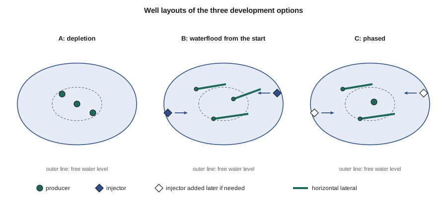
The afternoon ends with three options, each internally consistent and each the best of its kind.
| Option | Description | Capital (million US dollars) |
|---|---|---|
| A: depletion | Discovery well and two new vertical wells near the crest; no injection; battery and flowlines; gas gathered by a midstream company | 22.4 |
| B: waterflood from the start | Three horizontal producers high in the structure; 2-9 converted to injection and one new down-dip injector; battery with water injection | 41.4 |
| C: phased | Two horizontal producers and the discovery well; battery built ready for injection; after 18 months, add injection unless the aquifer has proved strong | 27.4 initially, plus 9.0 if injection is added |
The capital in the table excludes the discovery and appraisal wells. Their cost has been spent and cannot be recovered whatever the company decides, so it is sunk and irrelevant to the choice between options. The same principle applies to the extended test and the 3D survey. It is a principle that is easy to state and surprisingly hard to apply when a project has a history, because people naturally want to recover what they have spent. Daniel writes it into the economic basis so that no one is tempted.
Vertical or horizontal producers?
In a thin or low-permeability reservoir, horizontal wells are usually chosen because they contact far more rock than vertical wells. At Spruce Ridge the reservoir is thick and permeable, and productivity is not the problem. Water coning is. A vertical well perforated in the upper part of the oil column draws the pressure down most strongly around the wellbore, and if the drawdown is large enough, the oil-water interface below the well rises into a cone and water breaks through to the perforations. Above a critical rate the cone is unstable and water production starts early and grows. A horizontal well spreads the same production along a long section of wellbore, so the drawdown for a given rate is much smaller, and it can be placed high in the column, far from the water.
Hannah calculates the productivity of each well type and the critical rates. For the vertical well she uses the pseudo-steady-state radial inflow equation; for the horizontal well, Joshi's equation, which allows for the anisotropy between horizontal and vertical permeability. For the critical rate of a vertical well she uses the Meyer-Garder method, which balances the viscous pressure gradient toward the well against the buoyancy of the water. For the horizontal well she uses a screening estimate: the same critical drawdown, multiplied by the horizontal well's higher productivity.
# Well design screening: vertical and horizontal productivity, water-coning limits, and how many producers to drill.
import math
SI = False     # True: Canadian case (m, m3/d, Canadian dollars), False: US case (ft, bbl/d, US dollars)
FT, BBL = 3.2808, 6.2898
# reservoir and fluid data, held internally in oilfield units
if SI:
    k, kv_kh, h, col, mu, Bo, drho = 90.0, 0.3, 57 * FT, 67 * FT, 0.45, 1.45, 1.062 - 0.656
    re, rw, s, L = 400 * FT, 0.29, -1.0, 700 * FT
    N, netback, cap, qw = 1.825e6 * BBL, 300.0 / BBL, 320 * BBL, 160 * BBL  # P50 oil in place (bbl), net cash per bbl, facility and well limits
    wcost, fac, fixed = 8.4e6, 37.7e6, 1.8e6     # horizontal producer; facilities, injectors and pipelines; fixed cost per year
else:
    k, kv_kh, h, col, mu, Bo, drho = 45.0, 0.3, 80.0, 94.0, 0.40, 1.48, 1.080 - 0.668
    re, rw, s, L = 1500.0, 0.29, -1.0, 2600.0
    N, netback, cap, qw = 8.105e6, 32.0, 1600.0, 800.0
    wcost, fac, fixed = 6.8e6, 21.0e6, 1.5e6
show = (lambda q: f"{q / BBL:,.0f} m3/d") if SI else (lambda q: f"{q:,.0f} bbl/d")
showpi = (lambda j: f"{j / BBL * 0.145038:.2f} m3/d per kPa") if SI else (lambda j: f"{j:.1f} bbl/d per psi")
showdp = (lambda d: f"{d * 6.894757:,.0f} kPa") if SI else (lambda d: f"{d:,.0f} psi")

# vertical well, pseudo-steady state
Jv = 0.00708 * k * h / (mu * Bo * (math.log(re / rw) - 0.75 + s))
# horizontal well, Joshi (1988)
beta = math.sqrt(1 / kv_kh)
a = (L / 2) * math.sqrt(0.5 + math.sqrt(0.25 + (2 * re / L) ** 4))
Jh = 0.00708 * k * h / (mu * Bo * (math.log((a + math.sqrt(a * a - (L / 2) ** 2)) / (L / 2)) + beta * h / L * math.log(beta * h / (2 * rw))))
print(f"productivity index: vertical {showpi(Jv)}, horizontal {showpi(Jh)} ({Jh / Jv:.1f} times)")
dd = cap / 3
print(f"drawdown for {show(dd)} per well: vertical {showdp(dd / Jv)}, horizontal {showdp(dd / Jh)}")
# water coning: Meyer-Garder critical rate for a vertical well perforated in the top third of the oil column
hp = col / 3
qc_v = 0.001535 * drho * k * (col ** 2 - hp ** 2) / (mu * Bo * math.log(re / rw))
qc_h = qc_v * Jh / Jv                            # screening estimate: same critical drawdown, higher productivity
print(f"critical rate for water coning: vertical {show(qc_v)}, horizontal about {show(qc_h)} (screening estimate)")

# How many horizontal producers (with two injectors)? Reserves rise with diminishing returns; plateau is capped.
# Screening economics only: constant net cash per barrel after royalty and variable cost, fixed cost, no tax.
print(" n   EUR      plateau        capital   NPV10 (millions)")
best = None
for n in range(1, 7):
    eur = N * 0.40 * (1 - math.exp(-n / 1.5))  # recovery approaches 40 percent of oil in place
    plateau = min(cap, n * qw) * 365 * 0.95       # 95 percent uptime
    npv, Np, capex = 0.0, 0.0, fac + n * wcost
    for y in range(30):
        q = min(plateau, 0.20 * (eur - Np))
        if q * netback < fixed: break                # economic limit
        Np += q; npv += (q * netback - fixed) / 1.1 ** (y + 0.5)
    npv -= capex
    print(f"{n:2d} {eur / (1 if not SI else BBL) / 1e6:6.3f} {show(plateau / 365 / 0.95):>12s} {capex / 1e6:9.1f} {npv / 1e6:9.1f}")
    if best is None or npv > best[1]: best = (n, npv)
    last = npv
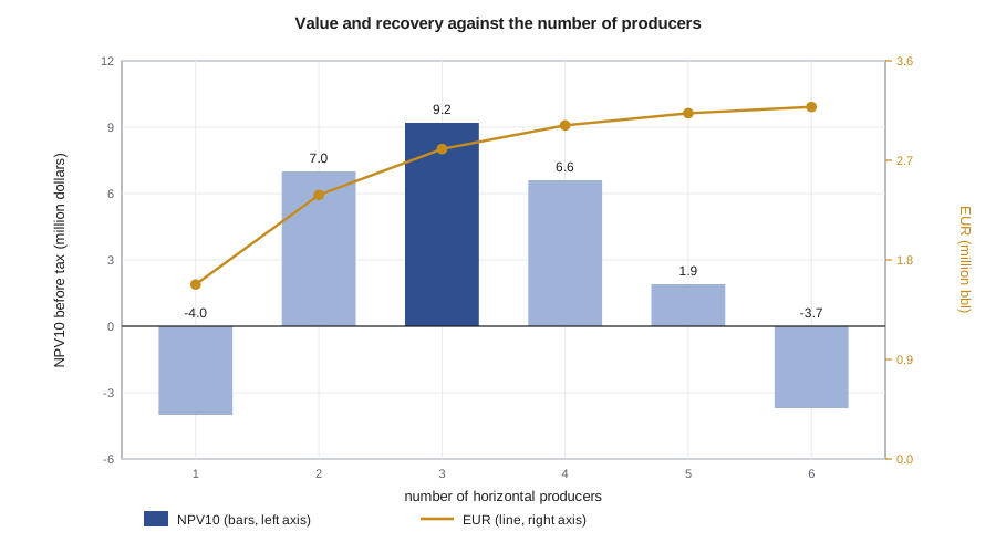
print(f"highest NPV10 with {best[0]} producers (EUR in million {'m3' if SI else 'bbl'})")productivity index: vertical 6.3 bbl/d per psi, horizontal 37.0 bbl/d per psi (5.8 times) drawdown for 533 bbl/d per well: vertical 84 psi, horizontal 14 psi critical rate for water coning: vertical 44 bbl/d, horizontal about 258 bbl/d (screening estimate) n EUR plateau capital NPV10 (millions) 1 1.578 800 bbl/d 27.8 -4.0 2 2.387 1,600 bbl/d 34.6 7.0 3 2.803 1,600 bbl/d 41.4 9.2 4 3.017 1,600 bbl/d 48.2 6.6 5 3.126 1,600 bbl/d 55.0 1.9 6 3.183 1,600 bbl/d 61.8 -3.7 highest NPV10 with 3 producers (EUR in million bbl)
The horizontal well is 5.8 times as productive as the vertical, and producing a third of the plateau rate takes a drawdown of only 14 psi compared with 84 psi for the vertical. Both are small, which confirms that productivity is not the constraint. The coning calculation is what matters: a vertical well can produce only about 44 bbl/d before water cones in, while a horizontal well placed high in the structure can produce about 260 bbl/d. Every well at Spruce Ridge will in practice produce above its critical rate, so water will come; the question is how soon and how much. Horizontal wells delay it substantially, which is why options B and C use them.
Critical-rate methods are conservative, because they treat the cone as stable and ignore the time it takes to form; in practice, most wells are produced above the critical rate and accept some water. They are useful here for comparison between well types rather than as rate limits. The team sets the design rate for each horizontal well at the level suggested by analog wells in similar carbonates, and uses the coning calculation to justify the choice of well type and the standoff from the free water level.
How many producers?
More wells recover more oil, faster, but each additional well adds less than the one before, because the wells share the same oil. The last part of the code screens the number of horizontal producers for the waterflood case, using a simple recovery model in which recovery approaches 40 percent of the oil in place as the number of wells increases, a plateau limited by the facility and by the rate per well, and a constant net cash flow per barrel after royalties and variable costs. It is a screening tool, not a forecast, but it captures the trade-off.
The NPV rises from one producer to two and to three, then falls: the fourth producer would add capital without adding enough oil or acceleration to pay for it. Even at its best, with three producers, the screening value is only about 9 million dollars against 41 million of capital, a first sign that the US case will be marginal. The team settles on three producers and notes that every million dollars of well or facility cost matters at Spruce Ridge.
Well design
Hannah drafts a basis of design for the producers. Each is drilled from a pad near the crest, built to horizontal within the upper third of the oil column, and drilled for about 2,600 ft through the best rock. The casing program follows the discovery well's, with an intermediate string set above the reservoir and a production liner, all in sour-service grades with controlled hardness, and premium threaded connections tested for gas tightness. The lateral is completed open hole or with a slotted liner, which is common in competent carbonate, and stimulated with an acid wash to remove drilling damage. The tubing, packer, wellhead and subsurface safety valve are all specified for sour service.
The injectors are simpler but have their own concerns. They are placed down-dip near the free water level so that the injected water supports the aquifer and pushes the oil up toward the producers, rather than cutting through the oil column to the nearest producer. Injected water must be compatible with the formation water and with the rock; incompatible waters can precipitate scale, such as barium or calcium sulfate, and plug the formation. The data acquisition plan already calls for a water analysis and compatibility test before the injection facilities are designed.
Worked problem
Standoff from the free water level
The oil column at the crest is 94 ft thick above the free water level. Hannah wants the horizontal laterals at least 60 ft above the free water level. If the crest is at 12,950 ft, what is the deepest the lateral can be placed, and how much room does that leave below the top of the reservoir?
Show solution
- The free water level is at 13,044 ft, so the lateral must be no deeper than 13,044 − 60 = 12,984 ft.
- At the crest that is 34 ft below the top of the reservoir; away from the crest the top dips and the window narrows.
- A lateral 2,600 ft long can follow the window only near the crest, so its trajectory must be designed on the depth map and steered with real-time logging.
Answer: The standoff limits where the laterals can go, and it is the reason three producers, not more, fit comfortably high on the structure.
Choosing the evaluation basis
The workshop ends with agreement on what will be compared. All three options use the same oil in place, the same aquifer cases, the same prices and the same cost database, so that the differences between them come only from the choices that define them. Option C is the most interesting: it buys flexibility. By delaying the decision on injection until 18 months of production have shown how the aquifer behaves, it avoids spending money on injection if the aquifer turns out to be strong, at the cost of a short delay if injection is needed. Whether that flexibility is worth its cost is a question for the economics in Lesson 10.
Common mistakes
MistakeIncluding sunk costs, such as the discovery and appraisal wells, in the comparison of options.
InsteadCompare options on future costs and revenues only; past spending is the same whatever is chosen.
MistakeChoosing horizontal wells because they are more productive, without asking what limits production.
InsteadIdentify the actual constraint; at Spruce Ridge it is water coning, not productivity.
MistakeUsing critical coning rates as hard rate limits.
InsteadTreat them as comparisons between designs; most wells produce above the critical rate.
MistakeDrilling the marginal well because recovery still increases.
InsteadAdd wells while the incremental value justifies the incremental capital and risk.
Summary and key terms
- Development options combine choices of recovery mechanism, wells, fluid handling and timing; each option should be internally consistent.
- Options that fail on feasibility, safety, economics or acceptability are screened out early, but the reasons are recorded.
- Sunk costs, such as the discovery and appraisal wells, are excluded from the comparison.
- In a thick, permeable carbonate, water coning rather than productivity limits vertical wells; horizontal wells high in the column delay water.
- The number of producers is set where the incremental value of a well no longer justifies its cost.
- Sour-service metallurgy, standoff from the free water level and injection water compatibility shape the well design.
- Development option
- A consistent combination of recovery mechanism, wells, facilities and timing.
- Sunk cost
- A cost already incurred that cannot be recovered and does not differ between options.
- Water coning
- Local rise of the oil-water interface toward a well caused by the pressure drawdown.
- Critical rate
- The highest production rate at which a stable cone does not reach the well.
- Marginal well
- A well whose incremental value is close to zero.
- Standoff
- The vertical distance between a well's completion and a fluid contact.
Practice problems
Work each problem on paper first, then reveal the answer to check.
Why is gas injection not a strong option at Spruce Ridge?
Show answer
The oil is far above its bubble point with no gas cap, and the sour gas has a market; injection would sacrifice revenue for little gain.
What limits the rate of vertical producers at Spruce Ridge?
Show answer
Water coning, not productivity.
Why should the cost of the discovery well be excluded when comparing options?
Show answer
It is sunk: it has been spent whatever option is chosen.
What does option C trade off?
Show answer
It saves the cost of injection if the aquifer proves strong, at the cost of a delay in injection if it does not.
Lesson quiz · 5 questions
Score 60% or more to complete this lesson.
Create a free account to save your progress, take quizzes and earn a certificate.