Reservoir simulation and history matching

Volumetrics say how much oil is in the rock. They say nothing about how it will come out. That depends on the energy available to push it to the wells, and at Spruce Ridge the energy question is the aquifer: how much water can flow into the pool from the surrounding rock as the pressure falls? The extended test is the only experiment that has been run on the reservoir. Mateo's job in weeks 6 to 8, the most critical activities on the schedule, is to build a model that reproduces the test, use it to estimate the aquifer strength, and forecast how the pressure would behave under each development option.

Which model?

Reservoir engineers have a hierarchy of models. At the simple end is the tank, or zero-dimensional material balance model, which treats the whole pool as a single volume with one average pressure and keeps track of the fluids produced, the fluids injected and the aquifer influx. At the complex end is the three-dimensional numerical simulator, which divides the reservoir into thousands or millions of cells, each with its own properties, and solves the flow equations between them. In between are analytical models for individual wells and simple layered or sector models.

The right model is the simplest one that answers the question with the data available. Spruce Ridge has two wells, four months of production from one of them and two months of shut-in. A full simulation model would have dozens of uncertain parameters that the data cannot constrain, and a history match with it would be hopelessly non-unique. A tank model has only a handful: the oil in place, the compressibilities, and the parameters of the aquifer model. The test data can constrain those. So Mateo builds a tank model for the history match and the pressure forecasts, and Connor builds a simple layered sector model that will be used later to test the effect of the tight layers on waterflood sweep. A full-field simulation model is listed as a define-stage deliverable, to be built when more wells and more production history exist.

Material balance above the bubble point

Material balance is conservation of mass applied to the reservoir as a whole. The reservoir volume of fluids withdrawn must equal the expansion of the fluids and rock left behind plus the water that flows in from the aquifer. Above the bubble point there is no free gas, and the test produced no water, so the balance in the form of Havlena and Odeh is:

where F is the underground withdrawal, N the oil in place, Eo and Efw the expansions of the oil and of the connate water and pore volume per unit of oil in place, We the cumulative water influx, and Δp the fall in average reservoir pressure. The expansion term is small. Even so, it determines how fast the pressure would fall without an aquifer: the effective compressibility is only a few millionths of the pore volume per unit of pressure.

For the aquifer, Mateo starts with the simplest model, Schilthuis's steady-state aquifer, in which the rate of influx is proportional to the pressure difference between the original aquifer pressure and the reservoir:

The constant Ja is the aquifer productivity index. A large value means an aquifer that responds strongly and quickly; a small value a weak one. More sophisticated models exist. The van Everdingen-Hurst model treats the aquifer as a radial or linear region and accounts for the time it takes for a pressure change to travel through it, and Fetkovich's pseudo-steady-state model treats it as a finite volume that loses pressure as it supplies water. Those models need the aquifer's size and permeability, which are not known. Over the four months of the test the steady-state model is a reasonable description of the near-field aquifer; whether it remains so over years is exactly the uncertainty the development plan must deal with.

History matching the extended test

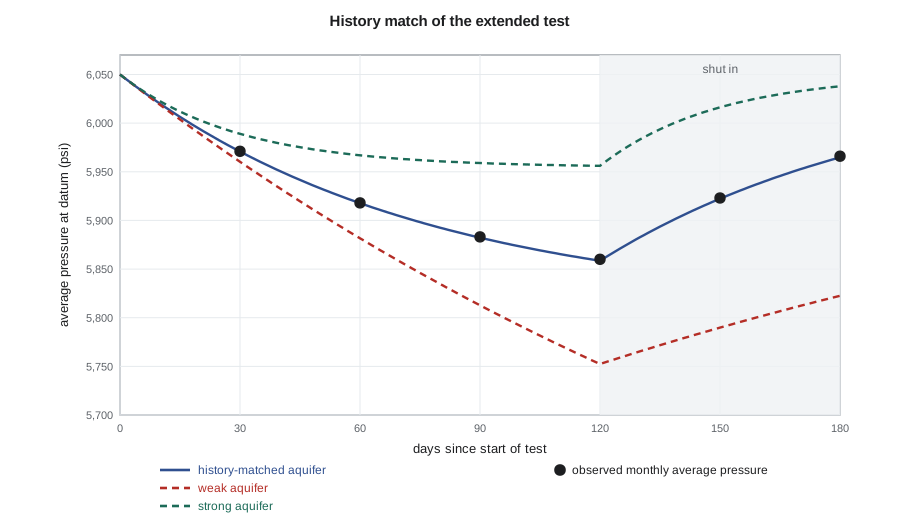
The history the model must reproduce is the average reservoir pressure at the end of each month: four months of production at a steady rate, followed by two months shut in. During production the pressure falls; during the shut-in it recovers as the aquifer keeps supplying water while nothing is being withdrawn. That recovery is the most valuable part of the record. A closed reservoir with no aquifer would show no recovery at all after shut-in, because nothing would refill it. A strong aquifer would refill it quickly. The shape of the drawdown and recovery together contains information about both the oil in place, which sets how much the pressure falls per unit withdrawn, and the aquifer strength, which sets how fast the pressure comes back.

# Tank material balance with a Schilthuis aquifer: history match of the extended test, then forecasts to the bubble point.
SI = False     # True: Canadian case (m3, kPa), False: US case (STB, psi)
if SI:
    pi, pb, Boi, co, Sw, cw, cf = 30850.0, 19400.0, 1.446, 1.91e-6, 0.14, 0.45e-6, 0.60e-6
    q_test, vu, pu, ju = 95.0, "m3", "kPa", "m3/(kPa d)"
    Ns = [1.505e6, 1.825e6, 2.211e6]            # P90, P50, P10 oil in place from Lesson 5
    obs = [30375, 30066, 29863, 29733, 30121, 30382]
    Js = [i * 0.005 for i in range(1, 81)]      # aquifer productivity index to search
    q_dev = 300.0                               # development plateau rate for the forecast
else:
    pi, pb, Boi, co, Sw, cw, cf = 6050.0, 3080.0, 1.477, 10.3e-6, 0.22, 3.0e-6, 4.0e-6
    q_test, vu, pu, ju = 420.0, "STB", "psi", "rb/(psi d)"
    Ns = [6.638e6, 8.105e6, 9.853e6]
    obs = [5971, 5918, 5883, 5860, 5923, 5966]
    Js = [i * 0.1 for i in range(1, 121)]
    q_dev = 1600.0
ct = co + (cw * Sw + cf) / (1 - Sw)              # expansion of oil, connate water and pore volume per unit of oil volume
sched = [(30, q_test)] * 4 + [(30, 0.0)] * 2     # four months of test production, then two months shut in

def tank(N, J, schedule, inj=0.0):
    """Daily steps. Returns month-end pressures. inj = water injection as a fraction of reservoir voidage."""
    p, We, Np, Wi, out = pi, 0.0, 0.0, 0.0, []
    for days, q in schedule:
        for _ in range(days):
            We += J * (pi - p)                   # Schilthuis steady-state influx, using yesterday's pressure
            Np += q; Wi += inj * q * Boi
            dp = (Np * Boi - We - Wi) / (N * Boi * ct - Np * Boi * co)
            p = pi - dp
        out.append(p)
    return out

def rms(N, J):
    return (sum((a - b) ** 2 for a, b in zip(tank(N, J, sched), obs)) / len(obs)) ** 0.5

print(f"effective compressibility {ct:.3e} per {pu}; observed month-end pressures {obs}")
best_all = None
for N, lab in zip(Ns, ("P90", "P50", "P10")):
    J = min(Js, key=lambda j: rms(N, j)); e = rms(N, J)
    print(f"{lab} oil in place {N / 1e6:.3f} million {vu}: best aquifer index {J:.3f} {ju}, RMS error {e:.1f} {pu}")
    if best_all is None or e < best_all[2]: best_all = (N, J, e)
N0 = Ns[1]
for J in (Js[0] * 6, Js[0] * 20, Js[0] * 50):
    print(f"   P50 with J = {J:.3f}: RMS error {rms(N0, J):.1f} {pu}")
Jm = min(Js, key=lambda j: rms(N0, j))
print(f"three-year forecast at {q_dev:,.0f} {vu}/d from the P50 tank:")
for name, J in (("weak aquifer", Jm / 3), ("history-matched", Jm), ("strong aquifer", Jm * 2.5)):
    p = tank(N0, J, [(30, q_dev)] * 36)
    m = next((i + 1 for i, x in enumerate(p) if x <= pb), None)
    pw = tank(N0, J, [(30, q_dev)] * 36, inj=0.9)[-1]
    print(f"  {name:15s} J = {J:6.3f}: no injection, " + (f"bubble point after {m} months" if m else f"{p[-1]:,.0f} {pu} after 36 months") +
          f"; 90 percent voidage replacement, {pw:,.0f} {pu}")

effective compressibility 1.627e-05 per psi; observed month-end pressures [5971, 5918, 5883, 5860, 5923, 5966]
P90 oil in place 6.638 million STB: best aquifer index 2.800 rb/(psi d), RMS error 12.2 psi
P50 oil in place 8.105 million STB: best aquifer index 2.600 rb/(psi d), RMS error 0.9 psi
P10 oil in place 9.853 million STB: best aquifer index 2.400 rb/(psi d), RMS error 11.4 psi
   P50 with J = 0.600: RMS error 120.4 psi
   P50 with J = 2.000: RMS error 25.6 psi
   P50 with J = 5.000: RMS error 55.0 psi
three-year forecast at 1,600 STB/d from the P50 tank:
  weak aquifer    J =  0.867: no injection, 3,263 psi after 36 months; 90 percent voidage replacement, 5,771 psi
  history-matched J =  2.600: no injection, 5,132 psi after 36 months; 90 percent voidage replacement, 5,958 psi
  strong aquifer  J =  6.500: no injection, 5,685 psi after 36 months; 90 percent voidage replacement, 6,014 psi

The P50 oil in place with an aquifer index of 2.6 rb/(psi·d) reproduces the six monthly pressures with a root-mean-square error of 0.9 psi, about the uncertainty of the pressure estimates. The P90 and P10 volumes can be matched only with errors of 11 to 12 psi, more than ten times larger, because the drawdown and recovery cannot both be fitted with the wrong oil in place. Aquifers much weaker or stronger than the matched value miss the data by tens to over a hundred psi. The test therefore supports both the volumetric P50 and a moderate aquifer, at least over the period observed.

How unique is the match?

A good match is not proof that the model is right. History matching is an inverse problem, and inverse problems are usually non-unique: different combinations of parameters can reproduce the same data. Here the team has been lucky, because the shut-in recovery separates the effect of the oil in place from that of the aquifer. But the match is conditional on the model. If the reservoir were compartmentalized, with the tight layers dividing it into partly connected parts, a smaller connected volume with a different aquifer might match equally well. If the aquifer were of finite size, it would behave like the matched steady-state aquifer for a few months and then weaken as its own pressure fell. Six months of data cannot tell those apart.

Mateo tests the first concern with Connor's layered sector model, which can include the tight layers as partial barriers. The test well's pressure response is almost unchanged unless the layers are made completely sealing over the whole pool, which the core and the well-test permeability-thickness agreement in Lesson 3 argue against. The second concern, aquifer size, cannot be tested with the data in hand. The regional maps show that the Red River water leg is connected to a much larger area, but faults and facies changes could limit the part that is in effective communication with the pool.

The team therefore carries three aquifer cases forward. The history-matched case uses the fitted index. The weak case uses one-third of it, representing an aquifer that is finite and starts to fail within a year or two of full production. The strong case uses two and a half times the fitted value, representing a larger and better connected aquifer than the short test could see. After discussion with Lena Haugen and Grace, the team assigns probabilities of 0.35, 0.45 and 0.20 to the weak, matched and strong cases. The probabilities are judgments, and the report says so, but they are written down and justified, which makes them open to challenge.

Forecasting the pressure

The last part of the output shows what each aquifer case implies for development. It runs the P50 tank for three years at the development plateau rate, first with no injection and then with water injected to replace 90 percent of the reservoir voidage.

With the weak aquifer and no injection, the pressure falls to 3,263 psi after three years, within 200 psi of the bubble point, after which solution-gas drive would take over and recovery would suffer. With the history-matched aquifer it falls to 5,132 psi, and with the strong aquifer it stabilizes near 5,685 psi. With 90 percent voidage replacement, the pressure stays within about 280 psi of the initial pressure in every case. The aquifer uncertainty that dominates the depletion forecast almost disappears once water is injected.

That is the key result of the history match, and it frames the whole development decision. Water injection is insurance against a weak aquifer. If the aquifer is strong, injection adds little and its cost is mostly wasted; if it is weak, injection is worth a great deal. The question for Lesson 10 is whether to buy the insurance now or wait to learn more about the aquifer first.

What the full simulation model will add

The tank cannot predict when water will break through at each well, how the water cut will rise, or how well a waterflood will sweep a layered reef. Those questions need a numerical model, and the define stage will build one: a geocellular model upscaled to a simulation grid of perhaps a hundred thousand cells, with relative permeability and capillary pressure from special core analysis and the aquifer represented numerically. The tank results set the targets that model must reproduce. Any full-field model whose average pressure did not match the extended test with the P50 oil in place and a similar aquifer would need explaining.

For the select stage, the team uses the tank results for pressure and combines them with recovery factors from analog pools and the sector model to estimate recovery under each option, as Lesson 8 shows. That is a standard approach at this stage, and the report says plainly that the waterflood recovery estimate relies on analogs and must be confirmed by simulation in the define stage.