Geological model and reservoir characterization

With the data checked, Connor turns to the geology. The geological model answers three questions that everything else depends on: how big is the container, how much of it is good rock, and how is the good rock arranged? The first sets the gross rock volume. The second, from logs and cores, sets the net-to-gross ratio, porosity and water saturation. The third, the arrangement of rock types and barriers, controls how the reservoir will produce: whether water from the aquifer will sweep it evenly or race along a few high-permeability layers, and whether a waterflood can reach the oil. Grace Nakoochee, who mapped the prospect, spends an afternoon with Connor and Mateo going through her interpretation.

The geological setting

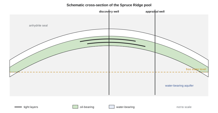
The Spruce Ridge pool is in the Ordovician Red River Formation, a carbonate unit that underlies the whole Williston Basin and has produced from structural traps in western North Dakota for decades. The productive interval, the Red River B zone, is a dolomitized burrowed limestone a few tens of feet thick, sealed above and below by dense limestone and anhydrite. At Spruce Ridge it is folded over a small structural high that was probably formed by movement on deep basement faults. The trap is a four-way closure: the reservoir rises to a crest and dips away on every side into the regional aquifer. Dolomitization created most of the porosity, including vugs, small cavities left where fossil fragments or earlier cements dissolved, and its intensity varies across the structure.

The setting matters for development. A carbonate reservoir is rarely a uniform tank. Grace's interpretation identifies three rock types. The first is a vuggy, coarsely crystalline dolomite with high porosity and permeability, which makes up most of the upper part of the reservoir. The second is a fine-crystalline dolomite with moderate porosity and much lower permeability. The third is dense, tight or shaly material that forms thin layers through the reservoir. Two such layers appear in the discovery well, and if they extend across the pool they could act as baffles to vertical flow, which would affect how the water from the aquifer rises and how a waterflood sweeps.

Mapping the container

The gross rock volume comes from the 3D seismic interpretation. Grace picked the top of the reservoir on the seismic volume, a reflection that ties well to the logs at both wells, and converted it from two-way travel time to depth with a velocity model calibrated at the wells. The depth map gives the area enclosed by each depth contour. The gross rock volume above the free water level is the integral of area over depth, which the team calculates with the trapezoidal rule from the area of each contour.

The largest uncertainty in the gross rock volume is not the integration but the depth conversion. Away from the two wells, the depth of the top of the reservoir depends on the velocity model, and an error of 1 percent in velocity over a depth of three kilometers or ten thousand feet is an error of tens of meters or feet in depth. At the edges of the structure, where the flanks dip gently, a small depth error moves the contour a long way laterally and changes the area substantially. Grace estimates that the depth uncertainty at the flanks is about plus or minus 6 m (20 ft), which is the main reason for the range of gross rock volume used in Lesson 5.

Petrophysics from the logs

The discovery well has a full suite of open-hole logs: gamma ray, bulk density, neutron porosity, sonic, deep and shallow resistivity and a borehole image. Connor computes porosity from the density log using a dolomite matrix density of 2.87 g/cm³ and a filtrate density of 1.00 g/cm³, checks it against the neutron and sonic logs, and computes shale volume from the gamma ray as a linear index between clean dolomite and the basinal shale. Water saturation comes from Archie's equation with formation water resistivity from the water sample recovered in the 2-9 well.

A sample is counted as net pay if it passes three cutoffs: porosity of at least 4 percent, water saturation no more than 50 percent, and shale volume no more than 30 percent. The cutoffs are not universal; they come from comparing core permeability with porosity in this rock, which shows that below about 4 percent porosity the dolomite has too little permeability to contribute to flow over the field's life. Cutoffs should be chosen before the calculation and tested for sensitivity afterwards, never adjusted to give a desired answer.

# Porosity, water saturation (Archie) and net pay from the discovery well logs, with a cementation-exponent sensitivity.
SI = False     # True: Canadian case (14-09, m), False: US case (1-9, ft)
if SI:
    step, du, rw = 3.0, "m", 0.035              # sample spacing, depth unit, formation water resistivity (ohm-m at reservoir T)
    # depth, gamma ray (API), bulk density (g/cm3), deep resistivity (ohm-m)
    log = [(3048, 18, 2.735, 558), (3051, 14, 2.694, 327), (3054, 12, 2.674, 262), (3057, 16, 2.705, 373),
           (3060, 22, 2.756, 776), (3063, 58, 2.805, 135), (3066, 15, 2.715, 418), (3069, 11, 2.661, 229),
           (3072, 13, 2.687, 298), (3075, 74, 2.825, 286), (3078, 15, 2.702, 346), (3081, 12, 2.681, 269),
           (3084, 14, 2.709, 358), (3087, 17, 2.722, 401), (3090, 19, 2.745, 511), (3093, 13, 2.696, 231),
           (3096, 12, 2.689, 173), (3099, 21, 2.737, 239), (3102, 15, 2.713, 113), (3105, 14, 2.704, 58.7),
           (3108, 18, 2.748, 57.0), (3111, 16, 2.719, 17.2), (3114, 17, 2.728, 8.4)]
else:
    step, du, rw = 5.0, "ft", 0.022
    log = [(12950, 16, 2.687, 189), (12955, 13, 2.644, 124), (12960, 11, 2.619, 101), (12965, 15, 2.661, 144),
           (12970, 66, 2.803, 80.0), (12975, 12, 2.633, 111), (12980, 10, 2.606, 89.1), (12985, 13, 2.649, 125),
           (12990, 15, 2.674, 154), (12995, 19, 2.705, 209), (13000, 12, 2.629, 90.5), (13005, 81, 2.829, 199),
           (13010, 14, 2.655, 85.6), (13015, 12, 2.640, 57.9), (13020, 15, 2.666, 51.3), (13025, 18, 2.689, 39.9),
           (13030, 13, 2.649, 14.7), (13035, 14, 2.662, 8.1), (13040, 16, 2.676, 4.1)]
rho_ma, rho_f = 2.87, 1.00                       # dolomite matrix and mud filtrate densities, g/cm3
gr_clean, gr_shale = 12.0, 110.0
a, n = 1.0, 2.0
phi_cut, sw_cut, vsh_cut = 0.04, 0.50, 0.30

def evaluate(m, show=False):
    gross = net = phih = hcph = 0.0
    for d, gr, rhob, rt in log:
        phi = max(0.0, (rho_ma - rhob) / (rho_ma - rho_f))
        vsh = min(1.0, max(0.0, (gr - gr_clean) / (gr_shale - gr_clean)))
        sw = min(1.0, (a * rw / (phi ** m * rt)) ** (1 / n)) if phi > 0 else 1.0
        pay = phi >= phi_cut and sw <= sw_cut and vsh <= vsh_cut
        gross += step
        if pay: net += step; phih += phi * step; hcph += phi * (1 - sw) * step
        if show: print(f"{d:7,.0f} {phi:6.3f} {vsh:5.2f} {sw:6.2f}  {'pay' if pay else '-'}")
    phi_av = phih / net; sw_av = 1 - hcph / phih
    return gross, net, phi_av, sw_av, hcph

print(f"  depth    phi   Vsh     Sw  ({du})")
gross, net, phi_av, sw_av, hcph = evaluate(2.0, show=True)
print(f"gross {gross:.0f} {du}, net pay {net:.0f} {du}, net-to-gross {net / gross:.2f}")
print(f"average porosity {phi_av:.3f}, average water saturation {sw_av:.3f}, hydrocarbon pore thickness {hcph:.2f} {du}")
for m in (1.8, 2.2, 2.4):                        # vugs raise m; fractures lower it
    g2, n2, p2, s2, h2 = evaluate(m)
    print(f"m = {m}: net {n2:.0f} {du}, Sw {s2:.3f}, hydrocarbon pore thickness {h2:.2f} {du} ({100 * (h2 / hcph - 1):+.0f} percent)")

# Gross rock volume above the free water level from the area enclosed by each depth contour (trapezoidal rule)
if SI:
    contours = [(3048.0, 0), (3050, 6), (3060, 28), (3070, 52), (3080, 78), (3090, 96), (3100, 115), (3110, 128), (3115.2, 131)]  # m, hectares
    grv = sum((a1 + a2) / 2 * 1e4 * (z2 - z1) for (z1, a1), (z2, a2) in zip(contours, contours[1:]))
    print(f"gross rock volume above the free water level: {grv / 1e6:.1f} million m3")
else:
    contours = [(12950.0, 0), (12960, 63), (12980, 207), (13000, 342), (13020, 450), (13040, 531), (13044.2, 545)]  # ft, acres
    grv = sum((a1 + a2) / 2 * (z2 - z1) for (z1, a1), (z2, a2) in zip(contours, contours[1:]))
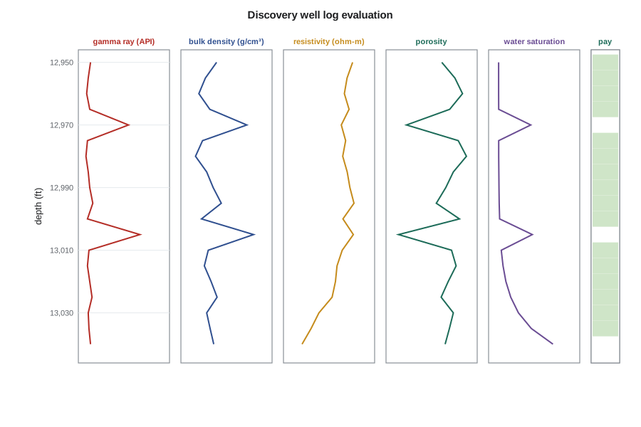
    print(f"gross rock volume above the free water level: {grv:,.0f} acre-ft")

  depth    phi   Vsh     Sw  (ft)
 12,950  0.098  0.04   0.11  pay
 12,955  0.121  0.01   0.11  pay
 12,960  0.134  0.00   0.11  pay
 12,965  0.112  0.03   0.11  pay
 12,970  0.036  0.55   0.46  -
 12,975  0.127  0.00   0.11  pay
 12,980  0.141  0.00   0.11  pay
 12,985  0.118  0.01   0.11  pay
 12,990  0.105  0.03   0.11  pay
 12,995  0.088  0.07   0.12  pay
 13,000  0.129  0.00   0.12  pay
 13,005  0.022  0.70   0.48  -
 13,010  0.115  0.02   0.14  pay
 13,015  0.123  0.00   0.16  pay
 13,020  0.109  0.03   0.19  pay
 13,025  0.097  0.06   0.24  pay
 13,030  0.118  0.01   0.33  pay
 13,035  0.111  0.02   0.47  pay
 13,040  0.104  0.04   0.71  -
gross 95 ft, net pay 80 ft, net-to-gross 0.84
average porosity 0.115, average water saturation 0.164, hydrocarbon pore thickness 7.72 ft
m = 1.8: net 80 ft, Sw 0.132, hydrocarbon pore thickness 8.01 ft (+4 percent)
m = 2.2: net 75 ft, Sw 0.179, hydrocarbon pore thickness 7.12 ft (-8 percent)
m = 2.4: net 70 ft, Sw 0.202, hydrocarbon pore thickness 6.45 ft (-16 percent)
gross rock volume above the free water level: 28,495 acre-ft

Over the 95 ft of gross reservoir above the free water level in the discovery well, 80 ft is net pay, a net-to-gross ratio of 0.84. The net pay has an average porosity of 11.5 percent and an average water saturation of 16.4 percent, giving a hydrocarbon pore thickness of 7.72 ft: if the oil in every pore were collected into a layer, it would be 7.72 ft thick. The two tight layers at 12,970 and 13,005 ft are excluded, and so is the bottom sample in the capillary transition just above the free water level. The gross rock volume from the depth map is 28,495 acre-ft, which the team rounds to 28,500.

The cementation exponent in vuggy rock

Archie's cementation exponent m describes how tortuous the conducting paths through the pore space are. For intergranular porosity it is close to 2. Vugs change that. A vug adds porosity but connects to the rest of the pore system only through the surrounding matrix, so it adds little to the electrical conductivity; the effective m rises, often to 2.2 to 2.5 or more in strongly vuggy rock. Fractures do the opposite and lower m. Using m = 2 in vuggy dolomite underestimates water saturation and overestimates oil in place.

The last lines of the output show how much this matters. With m = 2.2 the average water saturation rises from 16.4 to 17.9 percent and the hydrocarbon pore thickness falls by 8 percent; with m = 2.4 it falls by 16 percent and 10 ft of pay drops below the cutoff. The borehole image shows that vugs make up perhaps a fifth of the porosity in the upper part of the B zone, so Connor asks Mei Lin whether the core laboratory can measure m on plugs. It can, and the measured values, between 1.9 and 2.15 for most plugs, support using 2.0 with a modest allowance for uncertainty. The plugs with the most vugs gave 2.3, which the team keeps as the low case for saturation.

Permeability and rock types

Logs do not measure permeability. The team estimates it from a transform between core permeability and core porosity, fitted separately for each rock type because the same porosity in vuggy and fine-crystalline dolomite can mean permeabilities that differ by a factor of ten. The transform has the form log₁₀ k = aφ + b. The well test from the extended test gives an independent check: the permeability-thickness product from the buildup should be close to the sum of the core-derived permeability times thickness over the net pay.

From one well to the whole pool

The discovery well is near the crest, where the reservoir is thickest and the dolomitization most complete. The 2-9 well on the flank found a thinner section with more anhydrite and a net-to-gross ratio of only 0.46. The question is how to average the two across the pool. Grace's model, built from seismic amplitude, which here responds to porosity, puts the best dolomite over the crest and along a north-south trend. Weighting by volume, the team adopts pool averages of 0.62 for net-to-gross, 11.5 percent for porosity and 22 percent for water saturation, the last higher than at the crest because more of the pool's volume is near the free water level. These are the best estimates used in the volumetrics; Lesson 5 puts ranges around them.

Grace warns against one temptation. With only two wells, a geocellular model with millions of cells looks impressive but carries little more information than the two wells and the seismic. The team builds a simple layered model for the history match and forecasts and uses the detailed model only to test whether the tight layers, if continuous, would change the waterflood performance enough to matter. That question goes into the data acquisition plan: the first development well should be cored through the tight layers, and an interference test between wells would show whether they act as barriers.