
PET-499 · Lesson 10 of 12 · 20 min
Economics and decision analysis
Daniel has spent the term building the economic model in parallel with the technical work, with placeholder numbers that are now being replaced by the team's forecasts and costs. In week 12 the model has to answer the committee's question: which option creates the most value for Prairie Crest, how sure can the company be of that value, and what could make the answer wrong? Diane Mercer, who leads reserves and planning at Prairie Crest, reviews the model with him, and Graham Whitlock of Kestrel Petroleum Consultants, the company's reserves evaluator, has agreed to sit on the panel at the design review.
The economic basis
An economic evaluation is only as good as its assumptions, and the first thing any reviewer asks for is the basis: prices, costs, fiscal terms, discounting conventions and what is included or excluded. Daniel sets it out in one table at the front of the economics chapter, so that anyone can see it, challenge it, and rerun the model with a different assumption.
| Item | Assumption |
|---|---|
| Oil price at the field | 59 US dollars per barrel, flat in real terms, from Prairie Crest's planning deck |
| Gas and liquids | 2.40 US dollars per Mcf of raw gas, net of gathering, processing and sulfur handling fees |
| Operating cost | 1.5 million dollars per year fixed, 7 dollars per barrel of oil, 1 dollar per barrel of water handled |
| Royalty and production taxes | 3/16 (18.75 percent) lease royalty; North Dakota gross production and extraction taxes of 5 percent each on the working-interest share |
| Income tax | About 24 percent combined federal and North Dakota rate; intangible drilling costs and, with 100 percent bonus depreciation, tangible costs deducted when incurred; company is taxable |
| Discounting | Real terms, 10 percent, mid-year convention for production; capital at the time spent |
| Excluded | Discovery and appraisal wells, seismic and the extended test (sunk); corporate overhead |
| Abandonment | 0.35 million dollars per well plus 1.5 million for the facilities, at the end of life |
The royalty and tax terms are simplified, and the report says so. The actual royalty calculation works well by well, with each well's cost allowance depending on its depth and length, and the tax calculation would use the company's actual tax pools. For comparing options these simplifications are adequate, because they affect all options in the same way; for a sanction decision, the define-stage model will use the full terms. The assumption that the company is taxable matters: it means each dollar of deduction saves tax immediately against the company's other income, rather than being carried forward until Spruce Ridge itself makes a profit.
Cash flow and value for each option
For each option and aquifer case, the model takes the production forecast from Lesson 8, calculates revenue, royalties and operating costs year by year until the economic limit, when the field no longer covers its costs, and then adds the capital, the tax relief on it and the abandonment cost. It reports the net present value at 10 percent before and after tax, the internal rate of return, the payout time and the profit-to-investment ratio, defined here as the after-tax NPV10 divided by the discounted capital.
# After-tax economics of the three Spruce Ridge options, expected values over the aquifer cases, and the downside.
SI = False     # True: Canadian case (m3, Canadian dollars), False: US case (bbl, US dollars)
if SI:
    N, cap, qv, qh, gor = 1.825e6, 320.0, 90.0, 160.0, 150.0
    oil_p, gas_p = 500.0, 0.08                    # dollars per m3 of oil; net value per m3 of raw gas
    fixed, var, wat = 1.8e6, 45.0, 6.0            # dollars per year; per m3 oil; per m3 water
    tax, aband_w, aband_f = 0.23, 0.5e6, 2.5e6
    C_star, post = 6.0e6, 0.198                   # illustrative cost allowance per well; post-payout royalty rate
    capex = {"A": [(0.0, 11.6e6, 27.0e6)], "B": [(0.0, 32.4e6, 30.5e6)],   # (year, wells, facilities)
             "C": [(0.0, 17.8e6, 27.0e6)]}
    ph2_flood, ph2_strong = (1.5, 7.2e6, 4.0e6), (1.5, 0.0, 0.0)
else:
    N, cap, qv, qh, gor = 8.105e6, 1600.0, 450.0, 800.0, 900.0
    oil_p, gas_p = 59.0, 2.40e-3                  # dollars per bbl; net value per scf of raw gas
    fixed, var, wat = 1.5e6, 7.0, 1.0
    tax, aband_w, aband_f = 0.244, 0.35e6, 1.5e6
    capex = {"A": [(0.0, 10.4e6, 12.0e6)], "B": [(0.0, 26.4e6, 15.0e6)],
             "C": [(0.0, 14.4e6, 13.0e6)]}
    ph2_flood, ph2_strong = (1.5, 6.0e6, 3.0e6), (1.5, 0.0, 0.0)
RF = {"A": {"weak": 0.15, "matched": 0.25, "strong": 0.31}, "B": {"weak": 0.34, "matched": 0.35, "strong": 0.36},
      "C": {"weak": 0.32, "matched": 0.33, "strong": 0.345}}
wells = {"A": 3, "B": 5, "C": 5}
P_AQ = {"weak": 0.35, "matched": 0.45, "strong": 0.20}

def profile(opt, aq, Nf=1.0):                    # same model as Lesson 8
    eur = N * Nf * RF[opt][aq]; k = 0.28 if (opt == "A" and aq == "weak") else 0.20
    wmax = 0.40 if (opt == "A" and aq == "weak") else 0.85
    out, Np = [], 0.0
    for y in range(30):
        capy = 3 * qv if opt == "A" else cap if opt == "B" else 2 * qh + qv
        eur_y = N * Nf * 0.30 if (opt == "C" and y < 2) else eur
        q = min(min(capy, cap) * 365 * 0.95, k * (eur_y - Np))
        Np += q; wc = wmax * (Np / eur) ** 1.5
        out.append((q, q * wc / (1 - wc)))
    return out

def cashflow(opt, aq, Nf=1.0, price=1.0, cx=1.0):
    items = list(capex[opt])
    if opt == "C": items.append(ph2_strong if aq == "strong" else ph2_flood)
    rows, cum_rev = [], 0.0
    nprod = 3
    for y, (q, w) in enumerate(profile(opt, aq, Nf)):
        rev = q * oil_p * price + q * gor * gas_p * price
        if SI:                                    # 5 percent until revenue reaches the cost allowance, then post-payout rate
            below = max(0.0, min(rev, C_star * nprod - cum_rev)); roy = 0.05 * below + post * (rev - below); cum_rev += rev
        else:                                     # lease royalty, then production and extraction taxes on the remainder
            roy = rev * 0.1875 + rev * 0.8125 * 0.10
        opex = fixed + var * q + wat * w
        if rev - roy - opex <= 0: break
        rows.append((y + 0.5, rev - roy - opex))
    life = len(rows)
    # capital and tax relief (wells 30 percent and facilities 25 percent declining balance in Canada; expensed in the US)
    capital = [(t, -(wl + fc) * cx) for t, wl, fc in items]
    aband = [(life + 0.5, -(aband_w * wells[opt] + aband_f))]
    bt = rows + capital + aband
    shields = []
    for t0, wl, fc in items:
        if SI:
            for base, r in ((wl * cx, 0.30), (fc * cx, 0.25)):
                shields += [(int(t0) + yr + 1.0, tax * base * r * (1 - r) ** yr) for yr in range(30)]
        else:
            shields.append((t0 + 0.5, tax * (wl + fc) * cx))
    at = [(t, v * (1 - tax)) for t, v in rows] + capital + aband + shields
    return bt, at, life

npv = lambda fl, r=0.10: sum(v / (1 + r) ** t for t, v in fl)
def irr(fl):
    lo, hi = -0.5, 2.0
    for _ in range(80):
        mid = (lo + hi) / 2
        lo, hi = (mid, hi) if npv(fl, mid) > 0 else (lo, mid)
    return mid
def payout(fl):
    cum = 0.0
    for t, v in sorted(fl):
        cum += v
        if cum >= 0 and t > 0.4: return t
    return None

print(f"{'option':8s} {'NPV10 BT':>9s} {'NPV10 AT':>9s} {'IRR AT':>7s} {'payout':>7s} {'PIR':>5s}  (history-matched aquifer, millions)")
emv = {}
for opt in "ABC":
    bt, at, life = cashflow(opt, "matched")
    inv = sum(-v / 1.1 ** t for t, v in bt if v < 0 and t < 2)
    print(f"{opt:8s} {npv(bt) / 1e6:9.1f} {npv(at) / 1e6:9.1f} {100 * irr(at):6.0f}% {payout(at):6.1f}y {npv(at) / inv:5.2f}   life {life} years")
    emv[opt] = sum(P_AQ[a] * npv(cashflow(opt, a)[1]) for a in P_AQ)
print("expected NPV10 AT over the aquifer cases: " + ", ".join(f"{o} {v / 1e6:.1f}" for o, v in emv.items()))
for opt in "ABC":
    vals = [npv(cashflow(opt, a)[1]) / 1e6 for a in ("weak", "matched", "strong")]
    print(f"   {opt}: weak {vals[0]:.1f}, matched {vals[1]:.1f}, strong {vals[2]:.1f}")
print("downside and sensitivities, NPV10 AT (matched aquifer):")
for label, kw in (("P90 oil in place", dict(Nf=0.825)), ("price -25 percent", dict(price=0.75)), ("capital +25 percent", dict(cx=1.25))):
print(f" {label:20s} " + ", ".join(f"{o} {npv(cashflow(o, 'matched', **kw)[1]) / 1e6:.1f}" for o in "ABC"))option NPV10 BT NPV10 AT IRR AT payout PIR (history-matched aquifer, millions) A 17.6 12.8 47% 1.5y 0.57 life 11 years B 18.8 13.5 29% 2.5y 0.33 life 12 years C 19.9 14.4 37% 2.5y 0.41 life 12 years expected NPV10 AT over the aquifer cases: A 10.5, B 13.3, C 15.5 A: weak 1.1, matched 12.8, strong 21.8 B: weak 12.0, matched 13.5, strong 14.9 C: weak 13.1, matched 14.4, strong 22.3 downside and sensitivities, NPV10 AT (matched aquifer): P90 oil in place A 6.1, B 4.0, C 5.5 price -25 percent A 1.2, B -3.0, C -0.9 capital +25 percent A 8.5, B 5.5, C 7.6
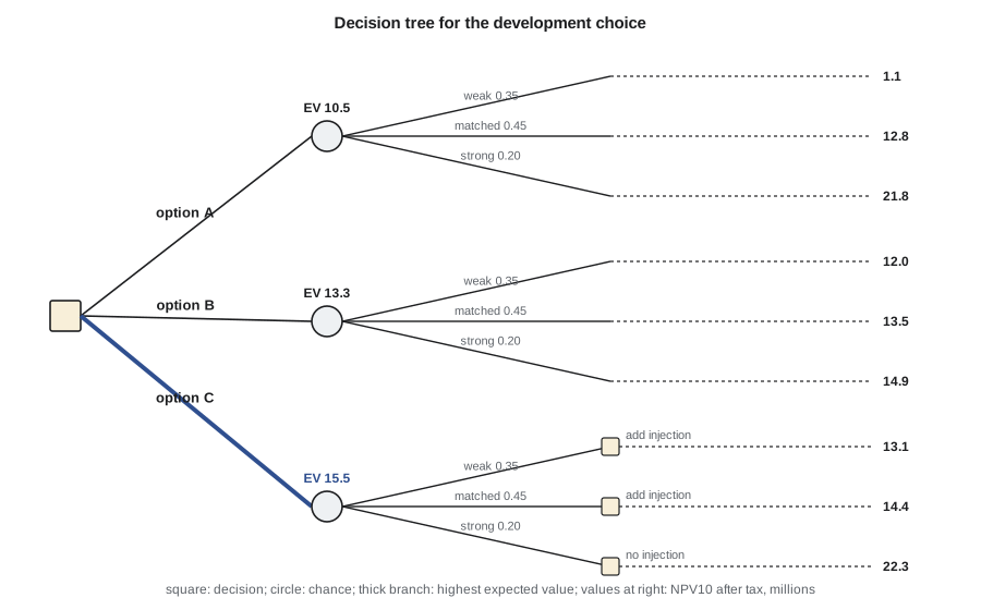
With the history-matched aquifer, all three options are economic, but none by much. Option C has the highest after-tax NPV10, 14.4 million dollars, ahead of option B at 13.5 million and option A at 12.8 million. The capital efficiency tells a sharper story: option A returns 0.57 dollars of NPV per dollar of discounted capital, option C 0.41 and option B 0.33. The expected values over the three aquifer cases, weighted 0.35, 0.45 and 0.20, put option C clearly first at 15.5 million dollars, followed by option B at 13.3 million and option A at 10.5 million. Option A's weakness is its weak-aquifer case, worth only 1.1 million; option C's strength is its strong-aquifer case, worth 22.3 million, where it avoids the cost of injection.
The value of flexibility
Option C is a real option in the sense used in finance: it gives the company the right, but not the obligation, to invest in injection later, after it has learned something. Its value comes from the ability to avoid a bad investment rather than from any better geology or engineering. The value of that flexibility is the difference between the expected value of the flexible option and that of the best rigid one. The decision tree makes it visible. In option B the company commits to injection now, whatever the aquifer turns out to be. In option C it waits 18 months, observes the pressure, and invests only if injection is needed.
Worked problem
How much would perfect knowledge of the aquifer be worth?
Suppose a perfect test could reveal the aquifer case before the company chooses an option. Using the NPVs from the output, find the expected value with perfect information and compare it with the best expected value without it.
Show solution
- Weak aquifer: best option is C at 13.1 million. Matched: C at 14.4 million. Strong: C at 22.3 million.
- Expected value with perfect information = 0.35 × 13.1 + 0.45 × 14.4 + 0.20 × 22.3 = 15.5 million dollars.
- The best choice without the information is option C, with an expected value of 15.5 million.
Answer: Perfect information about the aquifer would be worth essentially nothing. The reason is that option C is the best choice in every aquifer case, and by waiting to see the aquifer before investing in injection it already captures the value of knowing. Information is valuable only when it can change a decision, and here it would not.
That result answers a question Ethan had asked in week 6: should the company run a longer production test before deciding anything? With option C available, no. The development itself is the test. The permanent pressure gauge in the 2-9 well, recommended in Lesson 2, is what makes option C work: it provides the pressure history on which the phase 2 decision will be made, at a cost of a few tens of thousands of dollars.
The downside
Expected value is the right basis for a company that undertakes many projects, but a development committee also wants to know what happens if things go badly. The last part of the output tests three downside cases with the history-matched aquifer: oil in place at the P90 value from Lesson 5, a price 25 percent lower for the life of the field, and capital 25 percent above the estimate, the upper part of the class 4 accuracy range.
The downside cases are where the US Spruce Ridge project shows its weakness. At the P90 oil in place, the options are worth only 4.0 to 6.1 million dollars. With a 25 percent lower price, options B and C become negative, at −3.0 and −0.9 million, while option A, with the least capital, stays just positive at 1.2 million. A 25 percent capital overrun cuts option C to 7.6 million. The project creates value in the base case, but its margin for error is thin. The royalty and production taxes take about 27 percent of revenue before any costs, and the reserves are modest relative to the cost of three deep sour horizontal wells and a battery.
Risk, return and the choice
The economics give a more nuanced answer in the United States. Option C has the highest expected value and remains the best choice in every aquifer case. But option A, depletion with vertical wells, needs the least capital and is the only option that survives a sustained 25 percent fall in price, and a risk-averse committee could reasonably prefer it. Daniel's recommendation to the team is option C, with two conditions: that the company sanction it only after the gathering agreement with the midstream company is signed, which fixes the largest uncertain operating cost, and that the committee see the price sensitivity explicitly. Lesson 12 shows how the team presents that choice.
Daniel also checks the indicators against each other. The internal rate of return favors low-capital options, because it measures return per dollar rather than total value created; ranking by IRR alone would push the company toward option A and leave value in the ground. Payout favors options that produce quickly but says nothing about what happens afterwards. The NPV, expected over the uncertain cases and tested on the downside, is the measure that answers the committee's question. The other indicators describe the shape of the investment and are reported alongside it.
Common mistakes
MistakeRanking options by internal rate of return.
InsteadRank by expected NPV at the company's discount rate; use IRR, payout and PIR to describe the investment.
MistakeValuing a phased option as if the second phase were always carried out.
InsteadValue the decision at each branch; flexibility has value only because the second phase may not be needed.
MistakePaying for information that cannot change the decision.
InsteadCalculate the value of information first; with a flexible option it is often small.
MistakeReporting only the base case.
InsteadShow expected values over the uncertain cases and the downside cases the committee cares about.
Summary and key terms
- The economic basis, including prices, costs, fiscal terms, discounting and exclusions, must be stated explicitly and applied equally to all options.
- Sunk costs are excluded; the company's tax position affects the value of deductions.
- Expected NPV over weighted cases is the main measure of value; IRR, payout and PIR describe the investment's shape.
- A phased option is a real option whose value comes from avoiding unnecessary investment.
- The value of information is the gain from being able to change a decision; a flexible option can make it nearly zero.
- Downside cases at low volumes, low prices and high costs show how much margin a project has.
- Expected monetary value (EMV)
- The probability-weighted average of the values of the possible outcomes.
- Profit-to-investment ratio (PIR)
- NPV divided by discounted capital, a measure of capital efficiency.
- Payout
- The time for cumulative net cash flow to recover the capital.
- Real option
- The right, but not the obligation, to make a later investment decision after learning more.
- Value of perfect information
- The increase in expected value from knowing an uncertain outcome before deciding.
- Economic limit
- The point at which a field's revenue no longer covers its operating costs.
Practice problems
Work each problem on paper first, then reveal the answer to check.
Why are the discovery and appraisal wells excluded from the option comparison?
Show answer
They are sunk costs, the same whatever option is chosen.
Why might IRR favor option A even though it creates less value?
Show answer
IRR measures return per dollar invested, and option A uses the least capital.
What is the source of option C's advantage over option B?
Show answer
It avoids the cost of injection if the aquifer proves strong, while losing little if injection is needed.
When is information worth paying for?
Show answer
When it could change the decision and the expected gain exceeds its cost.
Lesson quiz · 5 questions
Score 60% or more to complete this lesson.
Create a free account to save your progress, take quizzes and earn a certificate.