
PET-360 · Lesson 9 of 12 · 19 min
Hydraulically fractured wells and rate-transient analysis
The company's Bakken wells are horizontal wells with 60 fracture stages each. The Tamarack 3-22H horizontal well has now produced for a year against a nearly constant flowing pressure, and nobody has shut it in, because a shut-in costs production and the buildup would take months to show anything useful. 'So we test it without stopping it,' Rafael says. 'The production data are a well test. The rate is the response and the pressure is held, which is just the problem turned around.'
This lesson covers the pressure behavior of hydraulically fractured wells, from single vertical fractures to multistage horizontal wells, and introduces rate-transient analysis (RTA), which applies well-test ideas to routine production data. In unconventional reservoirs, RTA is often the main source of reservoir information, because conventional buildups are impractically long.
A vertical well with one fracture
A hydraulic fracture creates a thin, highly conductive slot extending a half-length x_f on each side of the well. Two properties describe it: x_f, and the fracture conductivity k_f w_f, the product of the proppant pack permeability and the fracture width. Their combination with the reservoir permeability gives the dimensionless fracture conductivity, which decides how the fracture behaves.
When F_cD is large, above about 300, the fracture behaves as if it had infinite conductivity: the pressure drop along it is negligible, and early flow from the reservoir into the fracture faces is linear. Pressure change grows with the square root of time, and the derivative shows a half slope lying at half of Δp. When F_cD is small, the pressure drop along the fracture matters too. Then both the fracture and the reservoir have linear flow, at right angles, and the result is bilinear flow, where pressure grows with the fourth root of time and the derivative shows a quarter slope. Bilinear flow, when present, comes first and gives the conductivity; linear flow follows and gives x_f.
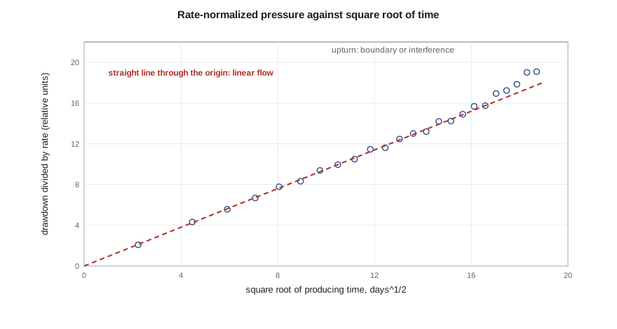
This is the linear-flow equation for an infinite-conductivity fracture in oilfield units. A plot of Δp against √t is a straight line through the origin, or through a small intercept if there is fracture-face skin, and its slope gives x_f√k. Note that the test gives the product, not each separately: a longer fracture in tighter rock and a shorter fracture in better rock can give the same linear-flow slope. The permeability must come from a radial-flow period, a pre-fracture test, or an independent estimate. After the linear period, the flow pattern becomes elliptical and finally pseudoradial; in pseudoradial flow, the fractured well behaves like an unfractured well with a strongly negative skin, typically between −3 and −6.
Multistage fractured horizontal wells
A horizontal well with many transverse fractures behaves, at first, like many fractured wells side by side. Each fracture drains the rock next to it, in linear flow. Once the pressure disturbances from neighboring fractures meet, the rock between them is depleted together, and the response looks like a closed box for a time. Later still, flow can come from the rock beyond the fracture tips, giving a compound linear flow perpendicular to the well, and in principle a final pseudoradial flow around the whole well. In tight rocks, that last regime can take decades to appear.
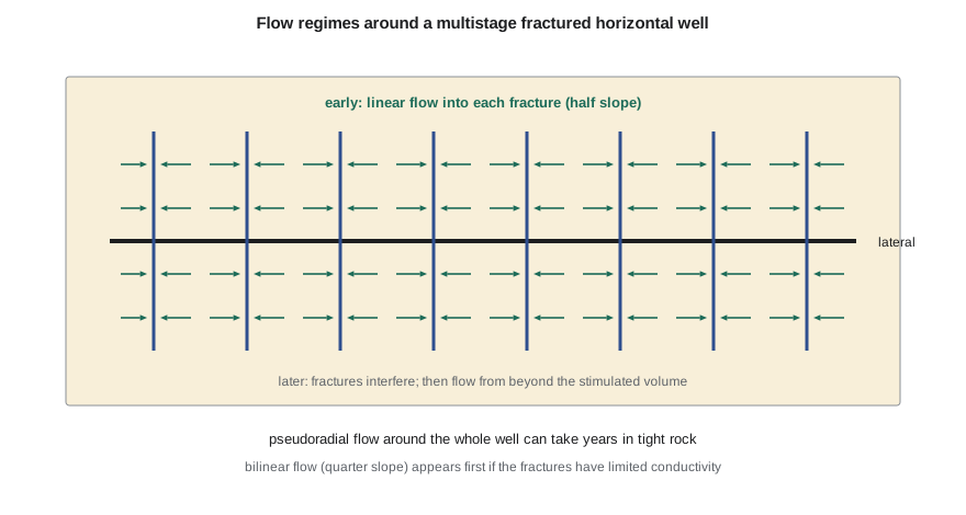
In this geometry, the total flow area is the sum of both faces of every effective fracture, A_c = 2 n x_f h for n fractures of half-length x_f in a layer of thickness h. The linear-flow analysis gives A_c√k. The words 'effective fracture' matter: not every stage creates a fracture that contributes, and fractures may be shorter or taller than designed. The analysis measures the combination that actually produces.
From pressure transients to rate transients
A well producing at constant flowing pressure has a declining rate. The mathematics is the mirror image of the constant-rate problem, and the main results carry over with modest changes. Wattenbarger and colleagues showed in 1998 that in linear flow the rate-normalized pressure, Δp/q, still grows with √t, but with a slope larger by a factor of about π/2 than in the constant-rate case. For variable rates and pressures, analysts use material-balance time, the cumulative production divided by the current rate, which converts a declining-rate history into an equivalent constant-rate history with good accuracy.
# Rate-transient analysis of a multistage fractured horizontal well in linear flow
import math
SI = False
DAY, MD = 86400.0, 9.869e-16                       # seconds per day; square meters per millidarcy
if SI:   # inputs in metric field units
    dp_kpa, B, mu_cp, phi, ct_kpa, h_m = 10000.0, 1.29, 0.72, 0.14, 1.5e-6, 6.5
    n_frac, xf_m, k_md = 40, 30.0, 0.5
    dp, ct, h, xf = dp_kpa * 1e3, ct_kpa / 1e3, h_m, xf_m
    qconv, qunit, afac, aunit = DAY, "m3/d", 1.0, "m2"
else:    # inputs in oilfield units
    dp_psi, B, mu_cp, phi, ct_psi, h_ft = 3870.0, 1.456, 0.40, 0.08, 1.5e-5, 45.0
    n_frac, xf_ft, k_md = 60, 250.0, 0.005
    dp, ct, h, xf = dp_psi * 6894.76, ct_psi / 6894.76, h_ft * 0.3048, xf_ft * 0.3048
    qconv, qunit, afac, aunit = DAY / 0.158987, "STB/d", 10.7639, "ft2"
mu, k = mu_cp * 1e-3, k_md * MD
Ac = n_frac * 2 * xf * h                            # flow area: both faces of every effective fracture
eta = k / (phi * mu * ct)
def rnp(t_days):                                    # constant-pressure linear flow: dp/q grows with sqrt(t)
    t = t_days * DAY
    return (math.pi / 2) * 2 * B * mu * math.sqrt(eta * t / math.pi) / (k * Ac)   # Pa per (m3/s)
print("  day   rate")
pts = []
for d in (5, 15, 30, 60, 90, 150, 240, 360):
    r = rnp(d); q = dp / r * qconv
    pts.append((math.sqrt(d), r)); print(f"{d:5d}  {q:7.1f} {qunit}")
# a straight line through the origin on dp/q versus sqrt(t) gives the slope; slope -> Ac*sqrt(k)
slope = sum(x * y for x, y in pts) / sum(x * x for x, _ in pts)   # Pa s/m3 per sqrt(day)
ac_sqrtk = (math.pi / 2) * 2 * B * mu * math.sqrt(1 / (math.pi * phi * mu * ct)) * math.sqrt(DAY) / slope
print(f"from the slope of dp/q against sqrt(t): Ac*sqrt(k) = {ac_sqrtk / math.sqrt(MD) * afac:.4g} {aunit}*sqrt(mD)")
print(f"with Ac = {Ac * afac:.4g} {aunit} from the completion design, k = {(ac_sqrtk / Ac) ** 2 / MD:.4f} mD")
print("halving the effective flow area would need four times the permeability: only Ac*sqrt(k) is unique") day rate
5 1571.1 STB/d
15 907.0 STB/d
30 641.4 STB/d
60 453.5 STB/d
90 370.3 STB/d
150 286.8 STB/d
240 226.8 STB/d
360 185.2 STB/d
from the slope of dp/q against sqrt(t): Ac*sqrt(k) = 9.546e+04 ft2*sqrt(mD)
with Ac = 1.35e+06 ft2 from the completion design, k = 0.0050 mD
halving the effective flow area would need four times the permeability: only Ac*sqrt(k) is uniqueThe synthetic 3-22H well starts at about 1,570 STB/d and declines to 185 STB/d after a year, a decline that follows the inverse square root of time almost exactly. The slope of Δp/q against √t gives A_c√k ≈ 9.5 × 10⁴ ft²·mD^½. With the designed flow area of 1.35 × 10⁶ ft², the permeability is 0.005 mD. Ethan's first instinct is to report that number, but Rafael points out that if only half the stages were effective, the same data would mean a permeability of 0.02 mD. Only the product is fixed by the data.
What RTA can and cannot tell you
A clear linear-flow period gives A_c√k and the time when linear flow ends. The end of linear flow, when fractures begin to interfere, gives a second relation: the time to the end is proportional to the square of the fracture spacing divided by the diffusivity. Together, the two can separate permeability from flow area, at least approximately. Before that, the answers are non-unique, and forecasts that assume a value for k or A_c should say so. Most RTA workflows also use the flowing material balance and type curves such as those of Fetkovich, Blasingame and Agarwal-Gardner, which plot normalized rate against material-balance time to identify regimes in the same way as the derivative in lesson 5.
RTA depends on data quality just as well testing does. Rates must be allocated accurately to each well, and flowing pressures should be bottomhole, either measured or calculated from wellhead pressure with a reliable flow correlation. Shut-ins for offset fracturing, artificial-lift changes and choke changes all disturb the record. In oil wells that produce below the bubble point, as most tight-oil wells do after a few months, the analysis should use multiphase corrections or pseudo-pressure, because the single-phase equations are only an approximation once free gas forms in the reservoir.
| Regime | Signature | Result |
|---|---|---|
| Bilinear flow | Quarter slope, Δp ∝ t^¼ | Fracture conductivity k_f w_f |
| Linear flow | Half slope, Δp ∝ √t | x_f√k, or A_c√k for a horizontal well |
| Fracture interference | End of linear flow; unit slope of a closed volume | Stimulated volume and fracture spacing |
| Compound linear flow | Second half slope | Flow from beyond the fracture tips |
| Pseudoradial flow | Flat derivative | kh and an equivalent negative skin |
Worked problem
Fracture half-length from a linear-flow slope
An older fractured vertical oil well in a partner's field, with data reported in oilfield units, has a linear-flow slope of 18 psi per root hour on a plot of Δp against √t. The rate is 150 STB/d, B = 1.3, μ = 1.1 cp, h = 40 ft, φ = 0.10, c_t = 1.5 × 10⁻⁵ psi⁻¹, and a pre-fracture test gave k = 0.3 mD. What is x_f?
Show solution
- The slope m_L = 4.064 qB/h × √(μ/(kφc_t)) / x_f.
- 4.064 × 150 × 1.3/40 = 19.8; √(1.1/(0.3 × 0.10 × 1.5 × 10⁻⁵)) = √(2.44 × 10⁶) ≈ 1,563.
- x_f = 19.8 × 1,563/18 ≈ 1,720 ft, far longer than the 800 ft design, so the inputs need checking.
- A typical cause is a permeability that is too low for the region the fracture drains; with k = 1.2 mD, x_f would be about 860 ft.
Answer: The arithmetic is simple, but the answer is only as good as the permeability used. An implausible half-length is a warning that k, or the assumption of a single planar fracture, is wrong.
Fracture tests before production: minifracs and DFITs
Much of what an engineer wants to know about a fractured well can be learned before the main treatment. In a diagnostic fracture injection test (DFIT), sometimes called a minifrac, a small volume of water is pumped into the formation fast enough to create a short fracture, and the pump is then stopped. The pressure falloff that follows passes through three stages. First, the fracture stays open and leaks fluid into the rock; the pressure falls along a characteristic curve that is analyzed with the G-function, a time function introduced by Nolte in the late 1970s. Second, the fracture closes; the closure pressure, read from the change in slope on a plot of pressure against the G-function or against the square root of time, is a good estimate of the minimum horizontal stress. Third, after closure, the pressure follows the reservoir's own response, first in linear flow and eventually in pseudoradial flow, from which permeability and reservoir pressure can be estimated.
In tight rock the after-closure period can last days or weeks, but because the injected volume is tiny, the well need not be produced, and a gauge left in place collects the data while the rest of the completion is planned. The closure stress guides the fracture design and the choice of proppant, and the permeability estimate removes some of the non-uniqueness of later rate-transient analysis, because it gives k independently of the flow area.
Fractured wells also bring a few practical hazards to testing. Proppant flowback can damage chokes and separators in the first days of production. Fracturing fluid returns carry chemicals, so flowback water is handled and disposed of under the operator's approvals. Pressure communication between a well being fractured and an older neighbor, often called a frac hit, can be recorded by gauges in the older well and gives a direct, if unwelcome, measure of how far the fractures reached.
Common mistakes
MistakeReporting k and x_f separately from linear flow alone.
InsteadLinear flow gives only x_f√k or A_c√k; another regime or independent data are needed.
MistakeUsing wellhead pressures directly.
InsteadConvert to bottomhole pressure, or measure it.
MistakeIgnoring the π/2 difference between constant rate and constant pressure.
InsteadUse the right linear-flow factor or material-balance time.
MistakeApplying single-phase equations far below the bubble point.
InsteadUse multiphase corrections or pseudo-pressure.
MistakeAssuming every stage is effective.
InsteadTreat A_c as unknown unless production logs or tracers say otherwise.
Summary and key terms
- Dimensionless fracture conductivity F_cD decides whether bilinear or linear flow appears first.
- Linear flow gives Δp proportional to √t and a half-slope derivative; the slope gives x_f√k.
- Multistage horizontal wells show linear flow into the fractures, then interference, then flow from beyond.
- RTA analyzes production at varying rate and pressure using rate-normalized pressure and material-balance time.
- At constant pressure, the linear-flow slope is about π/2 times the constant-rate slope.
- Linear flow alone leaves k and flow area non-unique.
- Fracture half-length x_f
- The distance from the well to the tip of one wing of a hydraulic fracture.
- Fracture conductivity
- The product of proppant pack permeability and fracture width, k_f w_f.
- Bilinear flow
- Simultaneous linear flow in the fracture and the reservoir, with Δp proportional to t^¼.
- Rate-transient analysis
- Analysis of production rates and flowing pressures using transient flow theory.
- Material-balance time
- Cumulative production divided by current rate.
- Fracture interference
- The stage at which the depleted regions of neighboring fractures meet.
Practice problems
Work each problem on paper first, then reveal the answer to check.
What does a quarter-slope derivative indicate?
Show answer
Bilinear flow in a finite-conductivity fracture.
What does the slope of Δp against √t give?
Show answer
x_f√k, or A_c√k for a multistage horizontal well.
Why is RTA used instead of buildups in tight rock?
Show answer
Buildups would take months and cost production.
What is material-balance time?
Show answer
Cumulative production divided by current rate.
Lesson quiz · 5 questions
Score 60% or more to complete this lesson.
Create a free account to save your progress, take quizzes and earn a certificate.