Buildup test analysis

After 48 hours of steady flow at 300 STB/d, Ethan has the lease operator close the Tamarack 7-15 well at the wellhead and leaves the downhole gauge recording for three days. The flowing pressure at shut-in is about 2,546 psi. 'Now you will see why everyone prefers buildups,' Rafael says. 'The rate is exactly zero, nobody is fiddling with a choke, and the gauge just listens to the reservoir.'

This lesson develops buildup analysis: superposition in time, the Horner plot, the extrapolated pressure p*, the simpler MDH buildup plot, the skin from a buildup, the effective producing time for wells with long and varying histories, and the step from p* to the average reservoir pressure used in material balance.

Superposition in time

Lesson 2 showed that a buildup can be built from two drawdowns. The well produces at rate q from time zero. At the shut-in time t_p, an imaginary well at the same location starts injecting at rate q, so that the net rate afterwards is zero. If Δt is the time since shut-in, the bottomhole pressure during the buildup is the initial pressure minus the effect of the producing well, which has now been flowing for t_p + Δt, plus the effect of the injector, which has been flowing for Δt.

The skin cancels out of the difference once the well is shut in, because both terms contain it. That is a useful result: after shut-in, the sandface rate is zero, so no pressure drop occurs across the damaged zone, and the buildup pressure reflects the reservoir alone. The skin enters only through the flowing pressure at the moment of shut-in, which is why the skin calculation in a buildup uses p_wf at Δt = 0.

The Horner plot

Substituting the logarithmic approximation for both p_D terms, the constants cancel and the buildup equation becomes very simple.

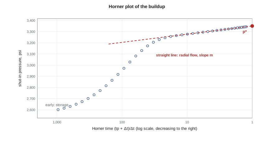
The quantity (t_p + Δt)/Δt is the Horner time ratio, after the engineer who published the method in 1951. On a plot of p_ws against the logarithm of the Horner time ratio, radial-flow data fall on a straight line with slope −m, the same m as in the drawdown. Horner time is large early in the buildup and falls toward one as Δt becomes very long, so the plot is usually drawn with the Horner axis increasing to the left, so that time runs left to right.

The slope gives kh exactly as in a drawdown: kh = 162.6 qBμ/m in oilfield units, or 2,149 qBμ/m in metric units. The rate q is the rate just before shut-in, and t_p is the producing time; for a well with a varying history, lesson notes below explain how to choose them.

The extrapolated pressure p*

Extending the Horner straight line to a Horner time of one, which corresponds to an infinitely long shut-in, gives a pressure called p*. In a truly infinite reservoir, p* equals the initial pressure p_i. In a new well or a newly opened zone, p* is therefore an estimate of the initial reservoir pressure, which is often the most valuable single number from a test.

In a reservoir that has been producing for some time, p* is not the average pressure, because the infinite-acting assumption no longer holds. Boundaries and neighboring wells have already depleted the drainage area. Matthews, Brons and Hazebroek (MBH) published charts in the 1950s that convert p* into the average drainage-area pressure for different drainage shapes and well positions, using the dimensionless producing time. An alternative, often attributed to Dietz, uses the shape factor and reads the average pressure from the semilog line at a particular shut-in time. Material balance (PET-320) needs the average pressure, so a buildup in a mature pool needs one of these corrections.

# Buildup test: Horner analysis after the drawdown, with superposition in time
import math
SI = False  
def E1(x):
    g, total, term = 0.5772156649, 0.0, 1.0
    for n in range(1, 60):
        term *= -x / n
        total += -term / n
    return -g - math.log(x) + total
if SI:   # metric units: m3/d, m, kPa, mPa.s, 1/kPa, h
    q, B, mu, h, phi, ct, rw, pi = 5.5, 1.29, 0.72, 6.5, 0.14, 1.5e-6, 0.089, 14090.0
    c_m, c_pD, c_tD, c_log, pu = 2149.3, 1866.6, 3.553e-6, -5.10, "kPa"
else:    # field units: STB/d, ft, psi, cp, 1/psi, h
    q, B, mu, h, phi, ct, rw, pi = 300.0, 1.25, 0.90, 30.0, 0.12, 1.2e-5, 0.35, 3350.0
    c_m, c_pD, c_tD, c_log, pu = 162.6, 141.2, 2.637e-4, -3.23, "psi"
k_true, s_true, tp = (15.0 if SI else 25.0), 5.0, 48.0      # tp: producing time before shut-in, h
def pD(t):
    return 0.5 * E1(1 / (4 * c_tD * k_true * t / (phi * mu * ct * rw ** 2))) + s_true
A = c_pD * q * B * mu / (k_true * h)
pwf0 = pi - A * pD(tp)                                     # flowing pressure at the moment of shut-in
def pws(dt):                                               # superposition: +q from t = 0, -q from t = tp
    return pi - A * (pD(tp + dt) - pD(dt))
print(f"flowing pressure at shut-in: {pwf0:.1f} {pu}")
print("  dt (h)   Horner time (tp+dt)/dt    pws")
rows = []
for dt in (1, 2, 4, 8, 12, 24, 36, 48, 72):
    ht = (tp + dt) / dt; p = pws(dt); rows.append((ht, p))
    print(f"{dt:7.0f}   {ht:14.2f}           {p:9.1f}")
pts = [(math.log10(ht), p) for ht, p in rows if ht < 8]     # late points, after storage
n = len(pts); sx = sum(x for x, _ in pts); sy = sum(y for _, y in pts)
sxx = sum(x * x for x, _ in pts); sxy = sum(x * y for x, y in pts)
slope = (n * sxy - sx * sy) / (n * sxx - sx * sx); icpt = (sy - slope * sx) / n
m = -slope                                                  # pressure rises as Horner time falls
k = c_m * q * B * mu / (m * h)
p1h = icpt + slope * math.log10(tp + 1)                     # the straight line at dt = 1 h
s = 1.1513 * ((p1h - pwf0) / m - math.log10(k / (phi * mu * ct * rw ** 2)) - c_log + math.log10((tp + 1) / tp))
print(f"Horner slope m = {m:.1f} {pu} per cycle, k = {k:.1f} mD")
print(f"p* (line extended to Horner time 1) = {icpt:.1f} {pu}")
print(f"p1h = {p1h:.1f} {pu}, skin s = {s:.2f}")

flowing pressure at shut-in: 2545.8 psi
  dt (h)   Horner time (tp+dt)/dt    pws
      1            49.00              3226.4
      2            25.00              3247.7
      4            13.00              3268.5
      8             7.00              3288.2
     12             5.00              3298.9
     24             3.00              3315.1
     36             2.33              3323.1
     48             2.00              3328.0
     72             1.67              3333.8
Horner slope m = 73.2 psi per cycle, k = 25.0 mD
p* (line extended to Horner time 1) = 3350.0 psi
p1h = 3226.4 psi, skin s = 5.00

The Horner fit gives a slope of about 73 psi per cycle, a permeability of 25 mD and a skin of +5.0, the same as the drawdown in lesson 3. The p* of 3,350 psi matches the starting pressure because the Tamarack 7-15 well has produced so little that the reservoir still behaves as infinite. Ethan notes that the buildup data are visibly smoother than the drawdown data, and that the first two hours, still under wellbore storage, lie well below the straight line.

Skin from a buildup

The skin follows from the flowing pressure at shut-in and the pressure on the straight line at one hour of shut-in.

The last term is small when t_p is much longer than an hour and is usually dropped. The metric version again replaces 3.23 with 5.10. As in the drawdown, p_1h is read from the straight line, not the data. The skin from a buildup is generally more reliable than from a drawdown because the shut-in data are cleaner, but it depends on an accurate flowing pressure at the instant of shut-in, which a downhole gauge records far better than a surface gauge.

The MDH buildup plot

When the producing time is much longer than the shut-in time, the Horner ratio (t_p + Δt)/Δt is close to t_p/Δt, and the buildup pressure becomes a straight line against log Δt alone. This plot, from the 1950 paper by Miller, Dyes and Hutchinson, is convenient for wells with long or poorly known production histories, because t_p does not appear. It is valid only while Δt remains small compared with t_p; late in a long buildup after a short flow, the MDH plot bends, while the Horner plot stays straight. For a short flow like the 48-hour flow in this test, Horner is the right choice.

Choosing the producing time

Real wells rarely produce at one constant rate before a buildup. A practical approximation, also due to Horner, replaces the actual history with a single rate equal to the last stable rate before shut-in and an effective producing time equal to the cumulative production divided by that rate: t_p = 24 N_p/q, in hours when N_p is in stock-tank barrels or cubic meters and q is in the matching unit per day. This works well when the last rate was held long enough to be stable. When the history includes large rate changes shortly before shut-in, the correct approach is full superposition of every rate change, which software handles routinely if the rate history is recorded.

A related trap is the length of the flow period itself. A buildup can only see what the flow period created. After a short flow, the buildup's radius of investigation is limited by the flow time as well as the shut-in time, and late buildup data after a short flow are dominated by the short producing history. A rule of thumb is to flow at least as long as the planned shut-in when boundaries or large distances matter.

Afterflow and phase redistribution

When a well is shut in at surface, the reservoir keeps feeding the wellbore until the wellbore pressure rises enough to stop it. This afterflow is the buildup form of wellbore storage, and it distorts the early data. In wells producing oil and gas together, a second effect called phase redistribution can occur: gas bubbles rise in the shut-in tubing, liquid falls, and the bottomhole pressure can rise and even hump above the reservoir trend before settling. Downhole shut-in tools prevent most of both effects. When they are not available, the derivative plot (lesson 5) shows where storage and redistribution end, so the straight line is fitted only to later data.