
PET-210 · Lesson 9 of 12 · 19 min
Subsurface maps, well logs and correlation
By the end of the first month, Ethan has digital logs from several hundred wells around Prairie Crest's acreage loaded into the team's mapping software, along with core descriptions from a dozen of them. The logs are a forest of wiggly curves. 'Every one of these wells cut the Bakken,' Nadia tells him. 'Your job is to pick the same surfaces in every well, so that when we draw a map, we are mapping the same thing everywhere.' Correlating wells and turning the picks into maps is the daily work of most petroleum geologists, and the maps are the foundation of every volume estimate and well plan.
Well logs for geologists
A well log is a continuous record of a rock property measured against depth, usually by tools lowered on a cable, called wireline logs, or carried in the drill string while drilling. PET-200 introduced the main logs; here the focus is on how geologists use them to identify rock types and correlate. Four logs do most of the work. The gamma-ray log measures natural radioactivity, which is high in shales because clay minerals hold potassium and thorium, and low in clean sandstones and carbonates. The resistivity log measures how strongly the rock resists electric current: salty water conducts, while oil, gas and dense rock do not, so high resistivity in a porous zone suggests hydrocarbons. The density and neutron logs estimate porosity and, together, distinguish rock types and gas.
The spontaneous potential (SP) log records small natural voltages caused by differences in salinity between the drilling mud and the formation water; it deflects opposite permeable beds and is useful in older wells that lack gamma-ray logs. The sonic log measures how fast sound travels through the rock and ties wells to seismic data. Image logs map the borehole wall in fine detail, showing bedding, fractures and sedimentary structures that indicate the direction of ancient currents. Each log responds to several rock properties at once, so geologists interpret them together and calibrate them against cores.
| Log | Measures | Main geological uses |
|---|---|---|
| Gamma ray | Natural radioactivity | Shale versus clean rock; correlation; grain-size trends |
| Spontaneous potential | Natural voltage from salinity contrast | Permeable beds; correlation in old wells |
| Resistivity | Resistance to electric current | Fluid type; hydrocarbon zones; correlation |
| Density | Bulk density from gamma-ray scattering | Porosity; lithology; seismic ties |
| Neutron | Hydrogen content | Porosity; gas detection with density |
| Sonic | Travel time of sound | Porosity; seismic velocity; overpressure |
| Image | Electrical or acoustic map of the borehole wall | Bedding dip, fractures, current direction |
Log shapes and facies
The shape of the gamma-ray curve through a sand body reflects how its grain size, and therefore its clay content, changes upward. A funnel shape, gamma ray decreasing upward, marks a coarsening-upward unit such as a shoreface or delta mouth bar. A bell shape, gamma ray increasing upward, marks a fining-upward unit such as a river channel or tidal channel fill. A blocky or cylinder shape, low and constant, marks a thick, uniform sand such as a stacked channel complex or an eolian dune. A serrated shape, alternating high and low, marks interbedded sand and shale. These patterns, calibrated with core, let geologists interpret depositional environments in wells that were never cored.
Geologists recognize key surfaces on logs too. A flooding surface often appears as an abrupt increase in gamma ray where shale sharply overlies sand, and the maximum flooding surface may show as a peak in gamma ray because organic-rich shale concentrates uranium. Sequence boundaries may be marked by a sharp base of a blocky sand cut into finer rocks, or by a change in the stacking pattern from coarsening-upward to fining-upward units. These surfaces, rather than the tops of individual sands, make the best correlation markers because they represent a single moment of time across the area.
Correlation
Correlation is the process of matching equivalent rock units or surfaces from well to well. Geologists hang logs side by side on a common datum, usually a widespread marker such as a flooding shale or a distinctive limestone, so that the correlation lines between wells are nearly horizontal and changes in thickness and facies are easy to see. Hanging on a datum removes the effect of later structure and shows the rocks roughly as they were deposited. The picks are then checked for consistency around loops of wells: a surface picked from well A to B to C and back to A must close at the same depth.
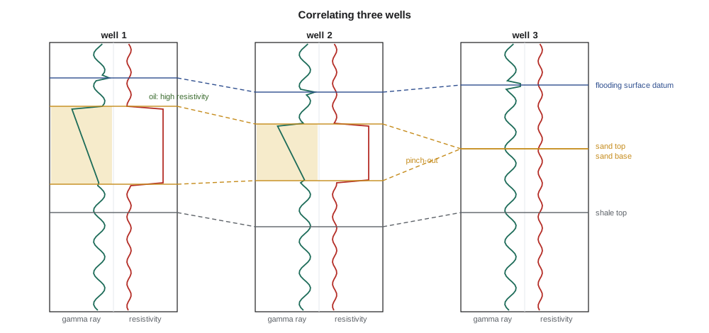
Two types of cross-section serve different purposes. A stratigraphic cross-section hung on a datum shows thickness and facies changes; a structural cross-section plotted at true depth below sea level shows the present shape of the layers, including folds and faults. Faults complicate correlation: a normal fault cutting a well removes part of the section, called a missing section, and a reverse fault repeats it. Recognizing missing and repeated sections helps geologists locate faults between wells and estimate their throw.
Subsurface maps
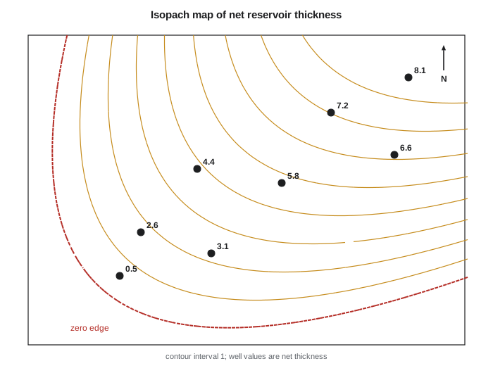
From the correlated picks, geologists make several kinds of maps. A structure map shows the depth, usually below sea level, of a surface such as the top of the reservoir, and defines traps, as Lesson 7 described. An isopach map shows the thickness of a unit, measured perpendicular to bedding; for gently dipping beds, the vertical thickness in a well is close enough. A net sand or net pay map shows the thickness of reservoir that passes the cutoffs of Lesson 3. Facies maps show where each rock type occurs. Property maps of porosity, water saturation or permeability show reservoir quality. Combining them gives the volume of the reservoir.
Contouring a map from scattered wells requires both technique and geology. Computer gridding algorithms estimate values at regular grid points from the nearby wells and then draw contours through the grid. Simple methods, such as inverse-distance weighting, average nearby wells with weights that fall off with distance. Kriging, a geostatistical method, uses the measured spatial correlation of the data to choose weights and also estimates the uncertainty at each point. But no algorithm knows that shoreface sands form belts parallel to the old coast or that a channel meanders. Geologists guide the contours with their depositional model, adding control points or editing the grid so that the map honors both the data and the geology.
# Gridding a net pay isopach from wells by inverse-distance weighting
# wells: (x miles east, y miles north, net pay ft)
wells = [(0.6, 0.6, 3.0), (1.6, 2.5, 11.0), (2.5, 1.2, 6.5), (3.1, 4.0, 15.0),
         (4.0, 2.5, 10.0), (4.7, 5.0, 16.0), (5.3, 3.4, 8.0), (1.9, 4.7, 13.0)]

def idw(x, y, p=2.0):
    num = den = 0.0
    for wx, wy, h in wells:
        d2 = (x - wx) ** 2 + (y - wy) ** 2
        if d2 < 1e-9: return h
        w = 1.0 / d2 ** (p / 2)
        num += w * h; den += w
    return num / den

for p in (1, 2, 3):
    print(f"power p = {p}: net pay (ft) on a 0.6-mile grid, north at top")
    for j in range(9, -1, -2):
        print("   " + " ".join(f"{idw(0.6 * i, 0.6 * j, p):5.1f}" for i in range(10)))
    acres_per_cell = 0.36 * 640
    vol = sum(idw(0.6 * (i + 0.5), 0.6 * (j + 0.5), p) * acres_per_cell for i in range(10) for j in range(10))
print(f" net pay volume over 36 square miles: {vol:,.0f} acre-ft\n")power p = 1: net pay (ft) on a 0.6-mile grid, north at top
11.0 11.2 11.5 11.8 11.9 12.0 12.2 12.7 13.3 12.3
10.7 10.9 11.3 11.8 12.1 13.2 12.3 11.9 11.6 11.1
10.1 10.2 10.5 10.7 10.8 11.0 10.8 10.6 10.2 9.7
8.9 9.0 9.3 9.4 9.2 9.5 9.9 10.1 10.1 10.2
7.0 3.0 7.3 8.3 8.5 8.9 9.4 9.7 9.9 10.0
net pay volume over 36 square miles: 241,652 acre-ft
power p = 2: net pay (ft) on a 0.6-mile grid, north at top
11.6 12.1 12.5 12.8 12.9 13.1 13.6 14.7 15.4 14.3
11.1 11.6 12.2 12.7 13.3 14.7 13.9 13.0 12.4 11.0
9.9 10.4 10.8 11.0 11.3 11.6 10.9 10.3 9.4 8.6
7.4 7.9 9.0 9.2 8.1 8.6 9.6 9.9 9.9 9.8
4.1 3.0 4.7 6.8 7.1 7.5 8.5 9.1 9.5 9.7
net pay volume over 36 square miles: 242,878 acre-ft
power p = 3: net pay (ft) on a 0.6-mile grid, north at top
12.2 12.6 12.9 13.0 13.2 13.7 14.6 15.6 15.9 15.3
11.6 12.1 12.7 13.0 13.7 15.0 14.7 13.8 12.9 10.5
10.0 10.6 10.9 11.0 11.6 12.1 10.7 10.1 8.8 8.1
6.3 7.3 9.3 9.3 7.4 7.8 9.5 9.9 9.8 9.5
3.2 3.0 3.6 6.1 6.6 6.9 7.7 8.7 9.2 9.5
net pay volume over 36 square miles: 243,624 acre-ftThe program grids reservoir thickness from eight wells, prints a small map for three values of the power p, and totals the volume. Inverse-distance weighting honors each well exactly but makes bull's-eye patterns around isolated wells and cannot extrapolate trends beyond them, which is why the edges of the map are poorly constrained. Changing the power p from 1 to 3 makes the map more local. Geologists treat machine-gridded maps as a starting point, then reshape them with the depositional trend, such as an old shoreline or channel belt, in mind.
Worked problem
Estimating a reservoir volume from an isopach map
Ethan's net pay map for a conventional sandstone prospect shows four contour bands: 0 to 3 ft covering 800 acres, 3 to 6 ft covering 520 acres, 6 to 9 ft covering 350 acres and 9 to 12 ft covering 150 acres. Estimate the net pay volume using the mid-point thickness of each band.
Show solution
- Band volumes: 1.5 ft × 800 acres = 1,200; 4.5 × 520 = 2,340; 7.5 × 350 = 2,625; 10.5 × 150 = 1,575 (all acre-ft).
- Total: 1,200 + 2,340 + 2,625 + 1,575 = 7,740 acre-ft of net pay rock.
- Average net pay over the 1,820-acre area: 7,740/1,820 = 4.25 ft.
Answer: About 7,740 acre-ft of net pay rock. Multiplying by 7,758 bbl/acre-ft, porosity and oil saturation, and dividing by the formation volume factor, gives the oil in place, as in PET-200.
Geosteering horizontal wells
Maps and correlations do not stop being useful once a field is drilled. In horizontal wells, geologists steer the bit through the reservoir in real time, a practice called geosteering. Logging-while-drilling tools send gamma-ray and resistivity readings to the surface every few seconds, and the geologist compares them with a model built from offset wells. If the gamma ray rises, the bit may be leaving the clean reservoir through its top or base; matching the pattern of the log to the expected layering tells which, and the directional driller adjusts the angle. Some tools measure resistivity around the borehole at a distance, mapping the boundaries of the layer several meters above and below the bit. In thin targets, such as a 3-meter shoreface sand or the middle member of a tight-oil play, good geosteering can keep a 3-kilometer lateral almost entirely in the best rock, which directly raises production.
Building the geological model
Modern studies combine maps, logs, cores and seismic into a three-dimensional geological model. The framework is built from mapped surfaces and faults, then divided into layers and filled with facies and rock properties using geostatistical methods that honor the well data and reproduce the patterns seen in cores and outcrops. Many equally plausible models, called realizations, are generated to capture uncertainty. The geological model is then upscaled to a coarser grid for reservoir simulation. The quality of every forecast depends on how well the correlation and mapping were done at the start, which is why experienced engineers spend time checking the geologist's picks rather than taking the model on trust.
Correlation is also where geologists and engineers most often disagree, productively. Production data can test a correlation: if two wells completed in what the geologist correlated as the same sand show different pressures, the correlation or the connectivity is wrong. Engineers who understand correlation can spot such contradictions early, and geologists who listen to engineering data build better models.
Common mistakes
MistakeCorrelating sand tops as if they were time lines.
InsteadSands can be diachronous or discontinuous; correlate flooding surfaces and sequence boundaries where possible.
MistakeAccepting machine-gridded maps without geological editing.
InsteadAlgorithms honor data but not depositional trends; guide contours with the facies model.
MistakeConfusing a missing section with thinning.
InsteadAn abrupt loss of section in one well can be a normal fault; check nearby wells and dipmeter data.
MistakeUsing structural cross-sections to study facies changes.
InsteadHang sections on a datum to remove later structure when studying stratigraphy.
Summary and key terms
- Gamma ray, resistivity, density, neutron, sonic and image logs identify rock types, fluids and surfaces; cores calibrate them.
- Gamma-ray log shapes, funnel, bell, blocky and serrated, indicate depositional environments.
- Correlation matches equivalent surfaces between wells, best done on time surfaces such as flooding surfaces, using a datum.
- Missing sections indicate normal faults and repeated sections indicate reverse faults.
- Structure, isopach, net pay, facies and property maps combine into reservoir volumes.
- Gridding algorithms such as inverse-distance weighting and kriging must be guided by geological models.
- Gamma-ray log
- A log of natural radioactivity, high in shale and low in clean sand or carbonate.
- Correlation
- Matching equivalent rock units or surfaces from well to well.
- Datum
- A reference surface used to align logs on a stratigraphic cross-section.
- Isopach map
- A map showing the thickness of a rock unit.
- Net pay map
- A map of the thickness of reservoir rock that passes porosity and saturation cutoffs.
- Missing section
- Part of the normal sequence absent in a well, often because a normal fault cuts it.
- Kriging
- A geostatistical gridding method that uses spatial correlation and estimates uncertainty.
Practice problems
Work each problem on paper first, then reveal the answer to check.
A gamma-ray curve through a sandstone increases steadily upward from low to high values. What environment might this indicate?
Show answer
A fining-upward unit, such as a river or tidal channel fill.
Why are flooding surfaces preferred over sand tops for correlation?
Show answer
They represent a single time across the area, while sand tops can be different ages and discontinuous.
A well is missing 25 m of section that is present in all neighboring wells. What is the likely cause?
Show answer
A normal fault with about 25 m of throw cuts the well.
Using inverse-distance weighting with p = 2, estimate thickness at a point 1 km from a well with 4 m and 2 km from a well with 8 m.
Show answer
Weights 1 and 0.25: (4 × 1 + 8 × 0.25)/(1.25) = 6/1.25 = 4.8 m.
Lesson quiz · 5 questions
Score 60% or more to complete this lesson.
Create a free account to save your progress, take quizzes and earn a certificate.