Inverse kinematics and the Jacobian

Robots are told where to go in the language of the task, not of their joints. The seal-face nest on the assembly fixture is at a position measured in the SCARA's base frame; the arbor on the balancing machine is a pose in R1's user frame. The robot controller must find joint angles that put the tool there. That reverse problem, inverse kinematics, is harder than forward kinematics because it may have several solutions, one, or none, and because near certain configurations small motions of the tool demand enormous joint speeds. This lesson works through inverse kinematics on robot R2, the SCARA that assembles seal faces, where the geometry is simple enough to solve by hand, then introduces the Jacobian, which relates joint speeds to tool speeds and reveals the configurations to avoid.

The SCARA

A SCARA, short for selective compliance assembly robot arm, has two parallel vertical revolute joints that move its arm in a horizontal plane, a vertical prismatic joint for lifting, and a rotation about the vertical at the tool. It is stiff vertically and slightly compliant sideways, which suits pushing parts into holes, and it is fast, often completing a standard pick-and-place cycle well under a second. R2 has an inner link of 325 mm and an outer link of 275 mm, for a reach of 600 mm. Its vertical and tool-rotation joints are independent of the planar ones, so the planar problem is a two-link arm, the classic starting point of inverse kinematics.

Solving the two-link arm

For a planar arm with links \(L_1\) and \(L_2\) and joint angles \(q_1\) and \(q_2\), the tip is at

Squaring and adding eliminates \(q_1\), because the distance from the base to the tip depends only on the elbow angle. By the law of cosines,

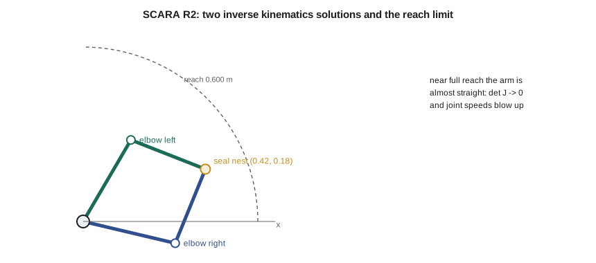
which gives two values of \(q_2\), one positive and one negative, for every reachable point: the elbow-right and elbow-left configurations. If the right-hand side exceeds 1 in magnitude the point is out of reach. With \(q_2\) known, the shoulder angle follows from the direction to the target less the angle the outer link adds: \(q_1 = \operatorname{atan2}(y, x) - \operatorname{atan2}(L_2\sin q_2, L_1 + L_2\cos q_2)\). The two-argument arctangent, atan2, matters: it returns the angle in the correct quadrant, where an ordinary arctangent of y/x would confuse opposite directions.

# Robot R2, a SCARA placing seal faces: inverse kinematics, the Jacobian and singularities
import math
L1, L2 = 0.325, 0.275       # link lengths (m); reach 0.600 m

def ik(x, y, elbow=+1):
    r2 = x * x + y * y
    c2 = (r2 - L1**2 - L2**2) / (2 * L1 * L2)
    if abs(c2) > 1: return None                       # outside the workspace
    q2 = elbow * math.acos(c2)
    q1 = math.atan2(y, x) - math.atan2(L2 * math.sin(q2), L1 + L2 * math.cos(q2))
    return q1, q2
def fk(q1, q2):
    return L1 * math.cos(q1) + L2 * math.cos(q1 + q2), L1 * math.sin(q1) + L2 * math.sin(q1 + q2)
def jac(q1, q2):
    s1, c1, s12, c12 = math.sin(q1), math.cos(q1), math.sin(q1 + q2), math.cos(q1 + q2)
    return [[-L1 * s1 - L2 * s12, -L2 * s12], [L1 * c1 + L2 * c12, L2 * c12]]

target = (0.420, 0.180)      # seal-face nest on the assembly fixture (m, in R2's base frame)
for elbow, name in ((+1, "elbow right"), (-1, "elbow left")):
    q1, q2 = ik(*target, elbow)
    x, y = fk(q1, q2)
    print(f"{name}: q1 {math.degrees(q1):7.2f} deg, q2 {math.degrees(q2):7.2f} deg  (check: x {x:.4f}, y {y:.4f} m)")

# Joint speeds needed to move the seal 0.25 m/s in +x, at the nest and near full reach
for pt in (target, (0.595, 0.0), (0.5999, 0.0)):
    q1, q2 = ik(*pt, +1)
    J = jac(q1, q2)
    det = J[0][0] * J[1][1] - J[0][1] * J[1][0]
    v = (0.25, 0.0)
    qd1 = (J[1][1] * v[0] - J[0][1] * v[1]) / det
    qd2 = (-J[1][0] * v[0] + J[0][0] * v[1]) / det
    print(f"at ({pt[0]:.4f}, {pt[1]:.3f}) m: det J = {det:.5f} m^2 (manipulability {abs(det):.5f}), "
          f"joint speeds {math.degrees(qd1):8.1f} and {math.degrees(qd2):8.1f} deg/s")
print("Target at 0.620 m:", "outside the workspace, no solution" if ik(0.62, 0.0) is None else "reachable")
print(f"Most dexterous elbow angle (largest |det J| = L1 L2 |sin q2|): q2 = 90 deg, |det J| = {L1*L2:.5f} m^2")

elbow right: q1  -13.29 deg, q2   81.13 deg  (check: x 0.4200, y 0.1800 m)
elbow left: q1   59.68 deg, q2  -81.13 deg  (check: x 0.4200, y 0.1800 m)
at (0.4200, 0.180) m: det J = 0.08831 m^2 (manipulability 0.08831), joint speeds     16.8 and    -68.1 deg/s
at (0.5950, 0.000) m: det J = 0.02291 m^2 (manipulability 0.02291), joint speeds    170.2 and   -371.9 deg/s
at (0.5999, 0.000) m: det J = 0.00327 m^2 (manipulability 0.00327), joint speeds   1202.8 and  -2624.4 deg/s
Target at 0.620 m: outside the workspace, no solution
Most dexterous elbow angle (largest |det J| = L1 L2 |sin q2|): q2 = 90 deg, |det J| = 0.08938 m^2

The nest at (0.420, 0.180) m can be reached elbow-right with \(q_1 = -13.29°\) and \(q_2 = 81.13°\), or elbow-left with \(q_1 = 59.68°\) and \(q_2 = -81.13°\). The program checks both by feeding them back through the forward kinematics, a habit worth keeping, since sign errors in inverse kinematics are common and the forward check catches them immediately. Which solution the robot uses is a programming choice. Most SCARA controllers let the programr specify the arm configuration, and moving between configurations requires the arm to pass through the straight-elbow position, which can sweep the outer link through space the programr did not expect. In BC-1, R2 works elbow-left at the nest because the elbow-right solution would bring the inner link close to the test fixture's guard.

Six-axis inverse kinematics

For a six-axis robot like R1, inverse kinematics is more involved, but industrial arms are designed to make it tractable. Their last three joint axes intersect at a single point, the wrist center. Given a tool pose, the wrist center is found by stepping back from the TCP along the tool's z axis by the tool length plus the flange offset. Its position depends only on the first three joints, which can be solved geometrically much like the two-link arm: joint 1 from the direction to the wrist center in plan, and joints 2 and 3 from a triangle in the vertical plane. The last three joints then supply the remaining orientation. Each stage has two solutions, front or back for joint 1, elbow up or down, wrist flipped or not, so a six-axis arm generally has up to eight solutions for one pose. Robot controllers handle the choice through configuration flags stored with each programd position, and a position taught in one configuration and replayed in another can produce an alarming move. Robots without a spherical wrist, such as some collaborative arms, need numerical solutions, iterative methods that start from a guess and refine it.

The Jacobian

Inverse kinematics finds joint positions for one pose. A robot moving along a straight line must also choose joint speeds at every instant, and the relation between joint speeds and tool speeds is the Jacobian matrix. For the planar arm,

Each column is the tool velocity produced by unit speed of one joint. To move the tool at a required velocity, the controller solves this system for the joint speeds, which requires J to be invertible. Its determinant for the two-link arm simplifies to \(L_1 L_2 \sin q_2\), which is zero when the elbow is straight or folded back, \(q_2 = 0\) or 180°. In those configurations the arm cannot move its tip along the line of the arm at all, however fast its joints turn: it has lost a degree of freedom. Such a configuration is a singularity. The magnitude of the determinant, sometimes called the manipulability measure, is largest at \(q_2 = 90°\), where the arm can move equally well in every direction.

The program shows what a singularity means in practice. Moving the seal face at 0.25 m/s in the x direction at the nest needs joint speeds of 16.8 and −68.1 degrees per second, easy for any SCARA. Near full reach at x = 0.595 m, where the arm is almost straight and the x direction points along it, the same tool speed needs 170 and −372 degrees per second. At x = 0.5999 m it needs 1,203 and −2,624 degrees per second, beyond any real motor. A controller following a straight line through such a point either slows the tool dramatically, stops with a fault, or, in older or simpler systems, lets the joints race. Robot programrs therefore keep straight-line moves away from the edge of the workspace, and integrators lay out cells so the working points sit comfortably inside reach. In BC-1, the nest is 457 mm from R2's base, about three quarters of its reach, where the manipulability of 0.0883 m² is close to the maximum of 0.0894 m².

Singularities of six-axis robots

Six-axis arms have three classic singularities, and anyone who programs or checks them should recognize all three. The wrist singularity occurs when axes 4 and 6 line up, which happens when joint 5 passes through zero; the controller cannot tell how to split a rotation between joints 4 and 6, and they may spin rapidly in opposite directions. The shoulder singularity occurs when the wrist center passes through the vertical line of joint 1, so the direction of joint 1 becomes undefined. The elbow singularity occurs at the edge of reach, when the arm is fully stretched. Look again at Lesson 8's working poses: joint 5 is at 60°, well clear of the wrist singularity, which was not an accident of the numbers. Simone's programrs chose the tool orientation to keep it there.

What the Jacobian also tells us

The same matrix relates forces as well as speeds. If the tool pushes on its surroundings with a force F, the joint torques needed to hold it are \(\tau = J^T F\). That is how a robot can estimate the force at its tool from its motor currents, and how force limits for collaborative operation are set; Lesson 11 uses it for payload checks. It also governs accuracy: a small joint angle error \(\delta q\) produces a tool error \(J \delta q\), which is the matrix version of the sensitivity calculated in Lesson 8. Near a singularity, where J is nearly singular, the reverse is also true: large tool-space corrections need large joint motions, so a controller using inverse kinematics to correct small errors there becomes unstable. Whether for speed, force or accuracy, the Jacobian is the single most useful object in robot kinematics.