Stability and the Routh criterion

Gilles has commissioned many pressure loops, and he tells Owen the story every controls technologist seems to have. On another test stand, years ago, a contractor tuned a pressure controller by turning up the gain until the response looked crisp. On the first test with a new pump, the drive began to surge, the discharge pressure swung between 1 and 5 bar every second, and the stand tripped on high pressure before anyone could reach the panel. Nothing was broken, but a pump under test had run through a damaging cycle of surges, and a customer witness had seen it. Feedback can make a stable process unstable. Before Owen proposes any gains for TL-3, Lucie wants him to know exactly where that boundary lies.

What stability means

A linear system is stable if every bounded input produces a bounded output; equivalently, its free response to any initial condition dies away. In terms of poles the condition is simple: a linear time-invariant system is stable if and only if every pole of its transfer function, the roots of its characteristic equation, has a negative real part. A pole on the imaginary axis gives a response that neither grows nor decays, a sustained oscillation or, at the origin, a constant drift; such a system is called marginally stable. A pole in the right half-plane gives a term that grows exponentially, and the system is unstable.

Open-loop, every plant in TL-3 is stable or, in the case of the integrating level and actuator processes, marginally stable. The question is what happens when the loop is closed. Closing a loop around G with a controller gain changes the characteristic equation from the plant's denominator to \(1 + K_cG(s)H(s) = 0\), and its roots move as \(K_c\) changes. For low gains they stay near the open-loop poles; as the gain rises, some of them may cross into the right half-plane.

Why feedback can destabilize

The physical reason is delay. Every lag in a loop makes the correction arrive late. A controller that pushes hard on an error it measured a moment ago may still be pushing after the error has reversed, so its correction feeds the next swing instead of opposing it. With enough gain and enough lag, the swings grow. The pressure loop has three lags in series, and at the frequency where together they delay the signal by half a cycle (180° of phase), negative feedback has become positive. If the loop gain at that frequency is one or more, an oscillation can sustain or grow itself. Lesson 11 develops this frequency-domain picture; this lesson finds the boundary algebraically.

The Routh-Hurwitz criterion

Finding the roots of a high-order polynomial was impractical before computers, and in 1877 Edward Routh published a test that tells how many roots lie in the right half-plane without finding them. It remains useful today because it gives stability conditions as inequalities in the parameters, which a root finder cannot do. For a characteristic polynomial

a necessary condition for stability is that all coefficients are present and have the same sign. If any is missing or negative, at least one root is not in the left half-plane. The necessary and sufficient test uses the Routh array. Its first two rows hold the coefficients, alternating:

and each later row is formed from the two above it in the same pattern: \(c_1 = (b_1a_{n-3} - a_{n-1}b_2)/b_1\), and so on, until a row for \(s^0\) is reached. The Routh-Hurwitz criterion states that the number of roots in the right half-plane equals the number of sign changes in the first column. The system is stable if and only if every entry of the first column is positive.

The pressure loop under proportional control

The pressure loop's characteristic equation with a proportional controller comes from Lesson 6:

For a cubic \(a_3s^3 + a_2s^2 + a_1s + a_0\), the first column of the Routh array is \(a_3,\; a_2,\; (a_2a_1 - a_3a_0)/a_2,\; a_0\). All coefficients are positive for any positive gain, so the only entry that can change sign is the third. Stability requires \(a_2a_1 > a_3a_0\):

The critical, or ultimate, gain is \(K_u = 23.5\). At exactly that gain, the \(s^1\) row is zero, and the \(s^2\) row then gives an auxiliary equation, \(a_2s^2 + a_0 = 0\), whose roots are the closed-loop poles on the imaginary axis: \(s = \pm j\sqrt{a_0/a_2} = \pm j\sqrt{a_1/a_3} = \pm 6.06j\) rad/s. The loop at the stability limit oscillates at 6.06 rad/s, a period of 1.04 s, which matches the one-second surging in Gilles's story uncannily well.

# Stability of the discharge pressure loop under proportional control: Routh array, critical gain and a check by simulation
import math
def routh(p):
    """Return the first column of the Routh array for polynomial p (highest power first)."""
    n = len(p); rows = [p[0::2], p[1::2] + [0.0]*(len(p[0::2]) - len(p[1::2]))]
    for _ in range(n - 2):
        a, b = rows[-2], rows[-1]
        piv = b[0] if b[0] != 0 else 1e-9          # epsilon method for a zero in the first column
        new = [(piv*a[i + 1] - a[0]*b[i + 1])/piv for i in range(len(a) - 1)] + [0.0]
        rows.append(new)
    return [r[0] for r in rows]
# Loop: Kc * 0.708 / ((0.5 s + 1)(0.72 s + 1)(0.1 s + 1)); characteristic equation a3 s^3 + a2 s^2 + a1 s + 1 + 0.708 Kc = 0
t1, t2, t3, Kp = 0.5, 0.72, 0.1, 0.708
a3 = t1*t2*t3; a2 = t1*t2 + t1*t3 + t2*t3; a1 = t1 + t2 + t3
print(f"Characteristic equation: {a3:.3f} s^3 + {a2:.3f} s^2 + {a1:.2f} s + (1 + {Kp} Kc) = 0")
for Kc in (4.0, 15.0, 30.0):
    col = routh([a3, a2, a1, 1 + Kp*Kc])
    changes = sum(1 for x, y in zip(col, col[1:]) if x*y < 0)
    print(f"  Kc = {Kc:5.1f}: first column {', '.join(f'{c:.3f}' for c in col)} -> {changes} sign change(s),"
          f" {'stable' if changes == 0 else 'unstable'}")
Kcrit = (a2*a1/a3 - 1)/Kp; wu = math.sqrt(a1/a3)
print(f"Critical gain Kcrit = {Kcrit:.1f}; oscillation at wu = {wu:.2f} rad/s, period Pu = {2*math.pi/wu:.2f} s")
print(f"Gain margin of the loop with Kc = 4: {Kcrit/4:.1f} ({20*math.log10(Kcrit/4):.1f} dB)")

# Simulate a 0.5 bar setpoint step near the limit to see the sustained oscillation
def sim(Kc, T=12.0, dt=0.0005):
    x = [0.0, 0.0, 0.0]; ys = []
    for n in range(int(T/dt)):
        u = Kc*(0.5 - x[2])                       # x[2] is the measured pressure deviation, bar
        x[0] += dt*(u - x[0])/t1                  # drive speed (scaled)
        x[1] += dt*(Kp*x[0] - x[1])/t2            # discharge pressure
        x[2] += dt*(x[1] - x[2])/t3               # transmitter output
        ys.append(x[2])
    tail = ys[len(ys)//2:]
    return max(tail) - min(tail)
for Kc in (10.0, Kcrit, 26.0):
    print(f"  Kc = {Kc:5.1f}: peak-to-peak swing in the second half of the run {sim(Kc):.3f} bar")

Characteristic equation: 0.036 s^3 + 0.482 s^2 + 1.32 s + (1 + 0.708 Kc) = 0
  Kc =   4.0: first column 0.036, 0.482, 1.034, 3.832 -> 0 sign change(s), stable
  Kc =  15.0: first column 0.036, 0.482, 0.452, 11.620 -> 0 sign change(s), stable
  Kc =  30.0: first column 0.036, 0.482, -0.341, 22.240 -> 2 sign change(s), unstable
Critical gain Kcrit = 23.5; oscillation at wu = 6.06 rad/s, period Pu = 1.04 s
Gain margin of the loop with Kc = 4: 5.9 (15.4 dB)
  Kc =  10.0: peak-to-peak swing in the second half of the run 0.008 bar
  Kc =  23.5: peak-to-peak swing in the second half of the run 0.831 bar
  Kc =  26.0: peak-to-peak swing in the second half of the run 2.855 bar

The program builds the Routh array at three gains. At \(K_c = 4\) and 15 every first-column entry is positive. At \(K_c = 30\) the third entry is −0.341, the column changes sign twice (positive to negative and back), and two roots are in the right half-plane, the complex pair that drives the growing oscillation. Simulations confirm the boundary: at \(K_c = 10\) the response settles, leaving a peak-to-peak ripple of only 8 mbar in the second half of the run; at 23.5 it oscillates with a steady swing of about 0.8 bar; at 26 the swing has grown to 2.9 bar and is still growing.

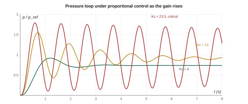
Relative stability and the gain margin

Being stable is not enough; a loop that is barely stable rings badly and becomes unstable when the plant changes slightly. The ratio of the critical gain to the gain actually used is the gain margin. At \(K_c = 4\), the pressure loop has a gain margin of 23.5/4 = 5.9, or 15.4 dB: the plant's gain could rise almost six-fold before the loop became unstable. That matters because the plant gain is not constant. Lesson 4 linearized it at full speed and 90 m³/h; at other test points the slope of pressure against speed differs, and a different pump on the stand has different curves. A common target is a gain margin of at least 2 (6 dB), and process engineers often prefer 3 or more.

The Routh test can also check how far into the left half-plane the poles sit. Substituting \(s = z - \sigma\) shifts the imaginary axis to the line \(\text{Re}(s) = -\sigma\), and applying the Routh test to the polynomial in z counts the roots to the right of that line. Requiring all closed-loop poles to have real parts below −0.4, for example, guarantees that every term decays at least as fast as \(e^{-0.4t}\), giving a settling time under about 10 s, the TL-3 specification.

Special cases

Two situations interrupt the construction of the array. If a first-column entry is zero but the rest of its row is not, replace the zero by a small positive number ε and continue; the signs of the remaining entries as ε tends to zero give the count. If an entire row is zero, the polynomial has roots symmetric about the origin, such as a pair on the imaginary axis. The auxiliary polynomial formed from the row above has those roots; differentiating it gives the coefficients to replace the zero row, and the construction continues. The pressure loop at its critical gain is an example of the second case.

The Routh test has limits worth knowing. It applies to polynomials, so a time delay must be approximated first, for example by a Padé form. It says whether a system is stable but not how well damped it is, except through the shifted-axis trick. And it applies to the linear model: a loop that is stable on paper can still oscillate if the real valve sticks or the drive saturates. Those effects return in Lesson 12.