
MEC-390 · Lesson 4 of 12 · 24 min
Electromechanical and multi-domain systems
The pressure loop of TL-3 crosses three energy domains before its output reaches the transmitter. The controller sends a speed reference to the variable frequency drive; the drive turns electrical power into torque in the motor; the motor spins the pump, which turns torque into head and flow; and the head pushes water through the pipe and valve, whose resistance and inertance set the discharge pressure. Owen's job this week is to link the pieces into one model and find out which of the many dynamics in that chain actually matter. The same week, Gilles asks him for a model of the hydraulic actuator of FV-301, a second multi-domain system in which electrical current becomes oil flow becomes stem motion.
Transducers between domains
Every multi-domain system contains transducers, elements that convert power from one domain to another. An ideal transducer stores nothing and loses nothing: power in equals power out. Two kinds cover almost every case. A transformer relates effort to effort and flow to flow in the same ratio, as a gear pair relates torque to torque and speed to speed, or a hydraulic piston relates pressure to force (\(F = pA\)) and flow to velocity (\(q = Av\)). A gyrator relates effort in one domain to flow in the other: a DC motor's torque is proportional to its current, \(T = K_t i\), and its back voltage to its speed, \(e = K_e\omega\). In SI units \(K_t = K_e\), which is the power balance written for an ideal motor.
Real transducers have losses and storage, which are modeled by adding resistances, capacitances and inertances on either side of the ideal element. A pump is a transducer from shaft power to hydraulic power whose ratio depends on speed and flow; it is described by its curves rather than by a single constant, and it must be linearized like any other nonlinear element.
The pump and the system
The TP-80's head curve at full speed, 1,760 rpm, is fitted closely by \(H = 40 - 12{,}800q^2\), with H in meters and q in m³/s. By the affinity laws of MEC-370, head at the same flow coefficient scales with the square of speed, so at a speed ratio \(r = n/1760\) the curve becomes \(H = 40r^2 - 12{,}800q^2\). The test loop's system curve has a static part of 23 m, set by the elevation of the return line and a back-pressure orifice, plus friction losses in the pipe and the throttling valve that rise with the square of flow: \(H = 23 + 14{,}400q^2\). The pump runs where the two curves cross.
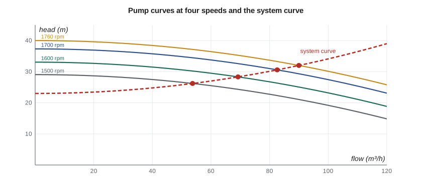
Setting the two expressions equal gives the flow \(q = \sqrt{(40r^2 - 23)/27{,}200}\) and then the head and discharge pressure. At full speed the pump delivers 90 m³/h at 32 m, a discharge pressure of 3.13 bar. At 1,500 rpm it delivers 54 m³/h at 2.57 bar; below about 1,330 rpm its shutoff head falls below the 23 m static head and no water passes at all. That last point matters for control: if the controller ever drives the speed below that value, the pump runs dead-headed and the pressure stops responding to speed, a nonlinearity that the linear model will not predict.
For the controller design, Owen needs the slope of discharge pressure against speed at the operating point. The program finds it by a central difference: 2.36 mbar per rpm, or 0.236 bar per 100 rpm. If the static head were zero, pressure would vary exactly with the square of speed and the slope would be \(2p/n = 3.56\) mbar/rpm; the static head flattens the relationship because part of the pressure is there regardless of speed.
The motor and the rotor
An induction motor on a fixed 60 Hz supply runs slightly below its synchronous speed of 1,800 rpm. In the normal operating range its torque is almost proportional to slip, the difference between synchronous and actual speed. The TP-80's motor delivers its rated 59.7 N·m at 1,760 rpm, a slip of 40 rpm, so near the operating point its torque falls by about 14.3 N·m for each rad/s of speed. The pump's torque rises with the square of speed, \(T_p = k\omega^2\), so its linearized slope is \(b_p = 2T_0/\omega_0 = 0.648\) N·m·s.
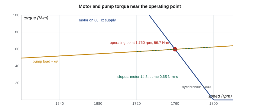
The rotor equation \(J\dot\omega = T_m(\omega) - T_p(\omega)\), linearized, becomes \(J\,d\Delta\omega/dt = -(b_m + b_p)\Delta\omega + \text{inputs}\), a first-order system with time constant \(\tau_m = J/(b_m + b_p)\). With J = 0.15 kg·m² for motor, coupling and wet pump rotor, \(\tau_m = 0.15/14.9 = 10\) ms. The motor's steep torque-speed curve acts like a very stiff speed regulator. This is the rotor's mechanical time constant on a fixed supply; on the drive, the drive's own speed controller makes the rotor follow its reference even more tightly, within limits of current and acceleration.
What the drive adds
A variable frequency drive changes the supply frequency to change the motor's synchronous speed. Modern drives run their own inner control loops on motor current and speed, sampled thousands of times a second, and present to the outside world a simple behavior: the motor speed follows the speed reference, subject to an acceleration ramp and a current limit. For TL-3, Gilles has set the ramp to 5 s from zero to full speed, 352 rpm/s. A 200 rpm change of reference therefore takes 0.57 s to complete, much longer than the 10 ms rotor time constant.
For small changes, Owen models the drive as a first-order lag with a time constant of 0.5 s, which matches the measured response of the old stand's drive to small steps and approximates the effect of the ramp. For large steps the ramp is a rate limit, a nonlinearity that the lag does not capture; the simulations in Lesson 12 include it explicitly. Either way, the conclusion is that the drive and its ramp, not the motor's physics, set the speed dynamics seen by the pressure loop.
# Multi-domain model of the TL-3 drive: induction motor on a VFD, the TP-80 pump and the loop, and the hydraulic actuator
import math
rho, g = 998.0, 9.81
# Pump and system curves at full speed (1,760 rpm): H in m, q in m^3/s
H0, a_p = 40.0, 12800.0         # shutoff head and curve coefficient: H = H0 r^2 - a_p q^2 (r = speed ratio)
Hs, a_s = 23.0, 14400.0         # system: static lift and back-pressure, plus losses a_s q^2
def operating_point(r):
    q = math.sqrt(max(H0*r*r - Hs, 0.0) / (a_p + a_s))
    return q, Hs + a_s*q*q
print(" speed (rpm)  flow (m^3/h)  head (m)  discharge (bar)")
for n in (1300, 1500, 1600, 1700, 1760):
    q, H = operating_point(n/1760)
    print(f"   {n:5d}       {q*3600:6.1f}      {H:5.1f}     {rho*g*H/1e5:5.2f}")
# Linearized gain of discharge pressure with speed at 1,760 rpm (central difference)
dn = 5.0
p_hi = rho*g*operating_point((1760+dn)/1760)[1]/1e5; p_lo = rho*g*operating_point((1760-dn)/1760)[1]/1e5
Kpn = (p_hi - p_lo) / (2*dn)
print(f"\nSmall-signal gain dp/dn = {Kpn*1000:.2f} mbar per rpm ({Kpn*100:.3f} bar per 100 rpm)")

# Rotor dynamics: J dw/dt = Tm(w) - Tp(w), both linearized at the operating point
J = 0.15                         # motor, coupling and pump with water, kg m^2
w0 = 1760*2*math.pi/60; T0 = 59.7
b_p = 2*T0/w0                    # pump torque ~ w^2, so dT/dw = 2T/w
b_m = T0 / (1800*2*math.pi/60 - w0)   # motor torque-slip slope on a fixed 60 Hz supply
tau_m = J / (b_m + b_p)
print(f"Pump load slope {b_p:.3f} N m s, motor slope {b_m:.1f} N m s, mechanical time constant {tau_m*1000:.1f} ms")

# On the VFD the speed follows the reference through the drive's own loop and a ramp limit
ramp = 1760 / 5.0                # rpm per s (0 to 1,760 rpm in 5 s)
print(f"Drive ramp: a 200 rpm step takes {200/ramp:.2f} s, much longer than the rotor time constant")

# Hydraulic actuator of FV-301: proportional valve flow into a cylinder
D, Vt, beta, mt = 0.050, 0.9e-3, 1.4e9, 22.0   # bore (m), total trapped oil (m^3), bulk modulus (Pa), moving mass (kg)
Ac = math.pi*D*D/4
Kq = 0.40e-3 / 10.0              # valve flow gain, m^3/s per V (0.40 L/s at 10 V)
print(f"\nCylinder area {Ac*1e4:.2f} cm^2; full-signal speed {Kq*10/Ac*1000:.0f} mm/s")
print(f"Position transfer function y/u = {Kq/Ac*1000:.1f}/s mm per V-s (an integrator)")
kh = 4*beta*Ac*Ac/Vt; wh = math.sqrt(kh/mt)
print(f"Oil spring stiffness {kh/1e6:.1f} MN/m, hydraulic natural frequency {wh:.0f} rad/s ({wh/2/math.pi:.0f} Hz)") speed (rpm) flow (m^3/h) head (m) discharge (bar)
1300 0.0 23.0 2.25
1500 53.7 26.2 2.57
1600 69.2 28.3 2.77
1700 82.6 30.6 2.99
1760 90.0 32.0 3.13
Small-signal gain dp/dn = 2.36 mbar per rpm (0.236 bar per 100 rpm)
Pump load slope 0.648 N m s, motor slope 14.3 N m s, mechanical time constant 10.1 ms
Drive ramp: a 200 rpm step takes 0.57 s, much longer than the rotor time constant
Cylinder area 19.63 cm^2; full-signal speed 204 mm/s
Position transfer function y/u = 20.4/s mm per V-s (an integrator)
Oil spring stiffness 24.0 MN/m, hydraulic natural frequency 1044 rad/s (166 Hz)Assembling the pressure loop model
The chain from speed reference to measured pressure now has four candidate dynamics: the drive (0.5 s), the rotor (0.01 s), the flow in the discharge line (0.72 s, from Lesson 3) and the pressure transmitter, which Gilles will set with a damping time constant of 0.1 s to filter turbulence noise. The rotor is fifty times faster than the drive and can be dropped. The other three are kept, with the static gain from the pump and system curves. Expressing the controller output and the measurement in percent, as industrial controllers do, makes the gain dimensionless: 1 percent of output is 18 rpm (the drive is scaled 0 to 1,800 rpm), and 1 bar is 16.7 percent of the transmitter's 0 to 6 bar span. The plant gain is therefore \(2.36 \times 10^{-3} \times 18 \times 16.7 = 0.708\) percent per percent.
Owen's model of the pressure process, to be written as a transfer function in Lesson 5, is a gain of 0.708 followed by three first-order lags of 0.5 s, 0.72 s and 0.1 s. It neglects the rotor, the torsional mode and the compressibility of the water, and it is linearized at full speed and 90 m³/h. Owen records all of these in the model's assumption list.
The hydraulic actuator
FV-301's actuator is a cylinder of 50 mm bore fed by a proportional directional valve. For small signals, the valve passes an oil flow proportional to its input voltage u: \(q = K_q u\), with \(K_q\) about 0.04 L/s per volt (0.40 L/s at the full 10 V). If the oil is treated as incompressible, all of that flow moves the piston, \(A_c\dot y = q\), so the stem velocity is proportional to the signal and the position is its integral:
With \(A_c = 19.6\) cm², full signal moves the stem at 204 mm/s. An actuator whose position is the integral of its input is an integrating process, and it behaves very differently from the self-regulating tank of Lesson 1: a constant small input does not lead to a new steady position but to steady motion until the stem hits its stop. Positioning such an actuator always needs a feedback loop, which Lesson 7 designs.
The oil is not truly incompressible. Trapped between the piston and the valve, it forms a spring with stiffness \(k_h = 4\beta A_c^2/V_t\) for a cylinder with equal volumes on each side, about 24 MN/m here. With the 22 kg of moving parts it gives a hydraulic natural frequency of 1,044 rad/s, or 166 Hz. That is far above the frequencies the position loop will use, so the integrator model is adequate, but it sets an upper limit on how fast the position loop can ever be made; a common rule is to keep the loop's bandwidth below about a third of the hydraulic frequency.
Worked problem
Speed of a larger actuator
A replacement valve for the larger TL-4 loop will need a cylinder of 63 mm bore. With the same proportional valve, what is the full-signal speed, and how long does a full 100 mm stroke take?
Show solution
- \(A_c = \pi(0.063)^2/4 = 3.12 \times 10^{-3}\) m².
- Full-signal speed \(= 0.40 \times 10^{-3}/3.12 \times 10^{-3} = 0.128\) m/s = 128 mm/s.
- Stroke time \(= 100/128 = 0.78\) s.
Answer: The larger cylinder is slower for the same valve. A 0.78 s stroke is still well inside the 5 s minimum closing time required to avoid water hammer, so the control system must limit the speed rather than the hardware.
Analogies
Because the element laws have the same form in every domain, systems in different domains with the same structure have the same equations. A mass-spring-damper, a pipe-tank-valve system and a series inductor-capacitor-resistor circuit all obey second-order equations of identical form. In the most common analogy, force corresponds to voltage and velocity to current, so a mass corresponds to an inductor, a spring to a capacitor of capacitance 1/k, and a damper to a resistor. The analogy is more than a curiosity: it means any technique learned in one domain, from transfer functions to Bode plots, works in all of them, and it lets engineers simulate mechanical and fluid systems with circuit tools.
| Mechanical (translational) | Mechanical (rotational) | Fluid | Electrical |
|---|---|---|---|
| force F | torque T | pressure p | voltage v |
| velocity v | angular speed ω | flow q | current i |
| mass m | inertia J | inertance I | inductance L |
| spring compliance 1/k | torsional compliance 1/kₜ | capacitance C | capacitance C |
| damper c | rotational damper b | resistance R | resistance R |
Common mistakes
MistakeKeeping every dynamic element in a multi-domain chain.
InsteadCompare time constants and drop those much faster than the loop.
MistakeUsing the pure square law for pressure against speed when there is static head.
InsteadFind the slope from the pump and system curves; static head flattens it.
MistakeModeling the drive as if the motor responded instantly to the reference.
InsteadThe drive's ramp and speed loop set the speed dynamics.
MistakeExpecting a hydraulic actuator to settle at a position for a constant input.
InsteadWith an ideal valve and cylinder, position is the integral of the input.
MistakeOperating a pump on speed control below the speed where shutoff head equals static head.
InsteadBelow that speed there is no flow and pressure no longer responds to speed.
Summary and key terms
- Transducers link domains; ideal ones conserve power, as transformers (gears, pistons) or gyrators (motors).
- TP-80 curves give operating points: 90 m³/h at 3.13 bar at 1,760 rpm, and no flow below about 1,330 rpm.
- The small-signal gain is 2.36 mbar/rpm, or 0.708 %/% in controller units.
- The rotor's time constant is 10 ms; the drive's ramp and speed loop, modeled as a 0.5 s lag, dominate.
- The pressure process is modeled as 0.708 with lags of 0.5, 0.72 and 0.1 s.
- The FV-301 actuator is an integrator, y/u = 20.4 mm/(V·s), with a hydraulic natural frequency of 166 Hz.
- Transducer
- An element that converts power from one energy domain to another.
- Transformer element
- A transducer relating effort to effort and flow to flow in a fixed ratio.
- Gyrator
- A transducer relating effort in one domain to flow in another, such as a DC motor.
- Slip
- The difference between synchronous and actual speed of an induction motor.
- Affinity laws
- Scaling rules relating pump flow, head and power to speed.
- Variable frequency drive
- An electronic controller that sets motor speed by changing supply frequency.
- Ramp limit
- The maximum rate at which a drive allows its speed to change.
- Integrating process
- A process whose output is the integral of its input and so has no natural steady state.
- Hydraulic natural frequency
- The resonance of a load on the oil spring of a hydraulic actuator.
- Analogy
- Correspondence between elements of different domains with equations of the same form.
Practice problems
Work each problem on paper first, then reveal the answer to check.
A DC motor has Kt = 0.5 N·m/A. What back voltage does it generate at 100 rad/s?
Show answer
Ke = Kt = 0.5 V·s/rad, so 50 V.
Using the TP-80 and system curves, find the flow at 1,650 rpm.
Show answer
r = 0.9375; q = √((40 × 0.879 − 23)/27200) = 0.0210 m³/s ≈ 76 m³/h.
Why can the rotor time constant be neglected in the pressure loop model?
Show answer
At 10 ms it is fifty times faster than the 0.5 s drive lag.
In the program, change the drive ramp to 10 s from zero to full speed. How long does a 200 rpm change take?
Show answer
The ramp becomes 176 rpm/s, so 1.14 s.
What full-signal speed does a 40 mm bore cylinder give with the same valve?
Show answer
A = 1.26 × 10⁻³ m²; 0.40/1.26 = 0.318 m/s.
In the force-voltage analogy, what corresponds to a pipe's inertance?
Show answer
Inductance.
Lesson quiz · 5 questions
Score 60% or more to complete this lesson.
Create a free account to save your progress, take quizzes and earn a certificate.