
MEC-390 · Lesson 7 of 12 · 20 min
First- and second-order time response
Farah's specification for TL-3 states its requirements in the language of time response. After a change of test point, the discharge pressure must settle within ±1 percent of the new value in less than 10 s. The throttling valve must reach a new position within 0.2 s and must not overshoot by more than 5 percent, because overshoot in valve position means a pressure spike. The suction level must stay within ±50 mm of its setpoint when the test flow changes. Before he can design controllers to meet these numbers, Owen needs to know exactly what they mean, how they relate to poles and gains, and how to read them from a test record.
First-order systems
A first-order system \(G(s) = K/(\tau s + 1)\) responds to a step of size A with
Its response has no overshoot and is completely described by two numbers: the gain K, which sets the final value, and the time constant τ, which sets the speed. At \(t = \tau\) the response has reached 63.2 percent of its final change; at 2τ, 86.5 percent; at 3τ, 95.0 percent; at 4τ, 98.2 percent. The 2 percent settling time is therefore about 4τ, and the 10 to 90 percent rise time is \(\tau\ln 9 = 2.2\tau\). The initial slope of the response is \(KA/\tau\), so a tangent drawn at the start meets the final value at exactly one time constant, a convenient way to estimate τ from a chart recording.
Many plants that are not truly first order behave nearly so, because one storage element dominates. The suction tank, the bearing frame and the flow in a long pipe are all modeled this way. The step test is the standard way to identify such a process: change the input suddenly, record the output and read off the gain and time constant.
Reading a step test: the bearing frame
Owen applies the method to the bearing frame record from the old stand, which logged a TP-80's frame temperature from a cold start at 21 °C. Six hours into the run the frame had settled at 60.6 °C. The gain is the change in output divided by the change in input: \(39.6/180 = 0.220\) K/W, matching the model of Lesson 3 exactly. The 63.2 percent point, 46.0 °C, falls at about 47 minutes on the record.
A single reading is sensitive to noise, so Owen also fits the whole early part of the record. Rearranging the first-order response gives \(\ln\big((T_\infty - T)/(T_\infty - T_0)\big) = -t/\tau\), a straight line through the origin with slope −1/τ. A least-squares fit of the first seven points gives τ = 46 minutes. The model of Lesson 3 predicted 49 minutes; the 6 percent difference most likely comes from the convection coefficient, which is hard to estimate for a finned casting. Owen updates the model to 47 minutes and moves on, since a controller tuned for one value will work perfectly well with the other.
# Time response: reading a first-order step test, and the second-order position loop of the valve actuator
import math
# 1. First order: identify K and tau from the logged bearing-frame warm-up (t in min, deg C)
log = [(0, 21.0), (10, 28.5), (20, 34.6), (30, 39.5), (45, 45.6), (60, 49.8), (90, 55.0), (120, 57.6), (180, 59.9), (240, 60.4)]
T0, Tinf = log[0][1], 60.6                     # start and settled value (from the 6-hour reading)
target = T0 + 0.632*(Tinf - T0)
for (t1, y1), (t2, y2) in zip(log, log[1:]):
    if y1 <= target <= y2: t63 = t1 + (target - y1)/(y2 - y1)*(t2 - t1); break
print(f"63.2 % point {target:.1f} deg C reached at t = {t63:.0f} min, so tau is about {t63:.0f} min")
print(f"Gain K = rise/heat = {(Tinf - T0)/180:.3f} K/W; 2 % settling time 4 tau = {4*t63/60:.1f} h")
# Log-linear fit: ln((Tinf - T)/(Tinf - T0)) = -t/tau, least squares through the origin
pts = [(t, math.log((Tinf - y)/(Tinf - T0))) for t, y in log[1:8]]
tau_fit = -sum(t*t for t, _ in pts) / sum(t*z for t, z in pts)
print(f"Least-squares fit of the early points: tau = {tau_fit:.0f} min")

# 2. Second order: P control of the FV-301 position loop. Plant y/u = Kv/(s (tv s + 1)), sensor 0.1 V/mm
Kv, tv, Ks = 20.4, 0.015, 0.1                  # mm/(V s), s, V/mm
def specs(Kc):
    wn = math.sqrt(Kc*Ks*Kv/tv); zeta = 1/(2*tv*wn)
    Mp = math.exp(-math.pi*zeta/math.sqrt(1 - zeta*zeta))*100 if zeta < 1 else 0.0
    return wn, zeta, Mp
def simulate(Kc, r=10.0, T=0.6, dt=1e-5):       # 10 mm setpoint step; states: position y (mm), valve flow term v
    y, v, out = 0.0, 0.0, []
    for n in range(int(T/dt)):
        u = Kc*Ks*(r - y)                       # controller output, V
        v += dt*(Kv*u - v)/tv; y += dt*v; out.append(y)
    peak = max(out); ts = next((k*dt for k in range(len(out) - 1, -1, -1) if abs(out[k] - r) > 0.02*r), 0.0)
    tr0 = next(k for k, val in enumerate(out) if val >= 0.1*r); tr1 = next(k for k, val in enumerate(out) if val >= 0.9*r)
    return max(peak/r - 1, 0.0)*100, (tr1 - tr0)*dt, ts
print("\n  Kc (V/V)   wn (rad/s)  zeta   Mp formula  Mp sim   rise 10-90 (ms)  settle 2 % (ms)")
for Kc in (5.0, 16.7, 40.0):
    wn, z, Mp = specs(Kc); Ms, tr, ts = simulate(Kc)
print(f" {Kc:6.1f} {wn:8.1f} {z:5.2f} {Mp:6.1f} % {Ms:5.1f} % {tr*1000:6.0f} {ts*1000:6.0f}")63.2 % point 46.0 deg C reached at t = 47 min, so tau is about 47 min
Gain K = rise/heat = 0.220 K/W; 2 % settling time 4 tau = 3.1 h
Least-squares fit of the early points: tau = 46 min
Kc (V/V) wn (rad/s) zeta Mp formula Mp sim rise 10-90 (ms) settle 2 % (ms)
5.0 26.1 1.28 0.0 % 0.0 % 183 332
16.7 47.7 0.70 4.6 % 4.6 % 45 125
40.0 73.8 0.45 20.4 % 20.4 % 21 113Second-order systems
The standard second-order system,
has poles at \(s = -\zeta\omega_n \pm j\omega_n\sqrt{1 - \zeta^2}\) when \(\zeta < 1\). Its unit step response, for \(K = 1\), is
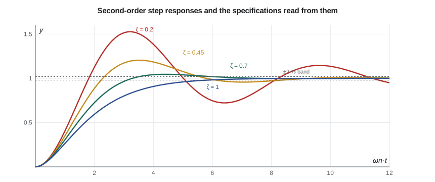
The damping ratio ζ alone sets the shape of the response; the natural frequency \(\omega_n\) only stretches or compresses it in time. Plotting the response against \(\omega_n t\) therefore gives a single family of curves, one for each ζ. Low damping gives a fast rise and large overshoot; ζ = 1 gives the fastest response without overshoot; larger ζ gives a sluggish, overdamped response.
Time-domain specifications
Five numbers describe a step response, and specifications are written in terms of them. The rise time \(t_r\) is the time to go from 10 to 90 percent of the final change. The peak time \(t_p\) is when the first maximum occurs. The percent overshoot \(M_p\) is how far the peak exceeds the final value, as a percentage of the change. The settling time \(t_s\) is the time after which the response stays within a band, usually 2 percent, of its final value. The steady-state error is the difference between the desired and actual final values. For the standard second-order system the first four have simple formulas:
The overshoot depends only on ζ: about 53 percent at ζ = 0.2, 20 percent at 0.45, 4.6 percent at 0.7 and none at 1. The settling time depends on the real part of the poles, \(\zeta\omega_n\), since that sets how fast the envelope decays. These relationships turn a specification into a region of the s-plane: an overshoot limit requires the poles to lie within a cone about the negative real axis (ζ above some value), and a settling-time limit requires them to lie to the left of a vertical line (\(\zeta\omega_n\) above some value). Lesson 10 uses exactly these regions to place closed-loop poles.
| ζ | Mₚ | tₛ ωₙ (2 %) | Typical use |
|---|---|---|---|
| 0.2 | 53 % | 20 | too oscillatory for most machines |
| 0.45 | 20 % | 8.9 | fast servos where some overshoot is tolerable |
| 0.7 | 4.6 % | 5.7 | a common design target |
| 1.0 | 0 | 5.8 | no overshoot allowed |
| 2.0 | 0 | 15 | sluggish; usually a sign of over-damping |
The valve position loop
The FV-301 actuator of Lesson 4 is an integrator, \(20.4/s\) mm per V·s. The proportional valve that feeds it is not instantaneous: its spool takes about 15 ms to respond, which adds a lag. The position sensor gives 0.1 V per mm (10 V over the 100 mm stroke). With a proportional controller of gain \(K_c\) acting on the position error in volts, the loop transfer function is \(L(s) = K_c(0.1)(20.4)/(s(0.015s + 1))\), and the closed loop is second order:
Raising the gain raises \(\omega_n\) but, because \(2\zeta\omega_n\) is fixed at 66.7 rad/s by the spool lag, it lowers ζ. To meet the 5 percent overshoot limit, ζ must be at least 0.69; choosing ζ = 0.7 gives \(\omega_n = 47.6\) rad/s and \(K_c = 16.7\) V/V. The program simulates a 10 mm step at three gains. At \(K_c = 16.7\), the overshoot is 4.6 percent, exactly as the formula predicts, the rise time is 45 ms and the response settles within 2 percent in 125 ms, inside the 0.2 s requirement. At \(K_c = 5\) the loop is overdamped and takes 330 ms to settle; at \(K_c = 40\) it rises faster but overshoots by 20 percent.
There is a second reason not to raise the gain further. The model neglects the hydraulic resonance at 1,044 rad/s found in Lesson 4. At \(K_c = 16.7\) the loop's natural frequency, 47.6 rad/s, is less than a twentieth of it, safely separated; much higher gains would bring the loop closer to the resonance and could make it unstable in a way the second-order model cannot predict.
Worked problem
Specification check for the pressure loop
With proportional control at \(K_c = 4\), Lesson 6 found closed-loop poles at −10.9 and \(-1.23 \pm 2.87j\). Treating the complex pair as dominant, estimate the overshoot and settling time, and compare with the specification of 10 s settling.
Show solution
- \(\omega_n = \sqrt{1.23^2 + 2.87^2} = 3.12\) rad/s; \(\zeta = 1.23/3.12 = 0.39\).
- \(M_p = 100e^{-\pi(0.39)/\sqrt{1 - 0.39^2}} = 26\) percent.
- \(t_s \approx 4/1.23 = 3.3\) s.
Answer: The loop settles well inside 10 s, but it overshoots by 26 percent of its change and, as Lesson 6 showed, settles 26 percent short of the setpoint. Speed is not the problem; overshoot and steady error are, and both call for a better controller than a proportional gain.
Higher-order systems and dominance
Real plants are rarely exactly second order, but their responses are often close to that of their dominant pair of poles. A pole whose real part is more than about five times that of the dominant pair decays so quickly that it barely affects the response, and it can be dropped, provided the DC gain is kept. The pressure loop at \(K_c = 4\) has its third pole at −10.9, nearly nine times as far from the axis as the complex pair, so the second-order estimates above are good. Zeros complicate the picture: a zero near the dominant poles adds overshoot and speeds the rise, and a zero in the right half-plane causes an initial dip. When in doubt, simulate.
Steady-state error to ramps
Steps are not the only test input. When a drive ramps the pump through a speed sweep, as during a full performance test, the pressure setpoint ramps too. A loop with one integrator, like the valve position loop, follows a ramp with a constant lag. For the position loop with \(K_c = 16.7\), the velocity error constant is \(K_v = 2.04K_c = 34\) per second, so a setpoint ramp of 20 mm/s is followed with a steady error of \(20/34 = 0.59\) mm. Lesson 9 generalizes this idea to the system type and the error constants.
Common mistakes
MistakeReading the time constant at 50 percent of the final value.
InsteadUse the 63.2 percent point, or fit the logarithm of the remaining error.
MistakeUsing second-order formulas for a loop whose third pole is close to the dominant pair.
InsteadCheck that other poles are at least five times further from the axis, or simulate.
MistakeRaising gain to speed up a loop without watching damping.
InsteadIn many loops, more gain lowers ζ and raises overshoot.
MistakeIgnoring neglected high-frequency dynamics when choosing gain.
InsteadKeep the loop's bandwidth well below resonances left out of the model.
MistakeMeasuring overshoot relative to the setpoint when the loop has steady error.
InsteadOvershoot is defined relative to the final value of the response.
Summary and key terms
- A first-order step response reaches 63.2 percent at τ and settles within 2 percent in about 4τ.
- The bearing frame's record gives K = 0.220 K/W and τ ≈ 46 to 47 minutes, close to the model's 49 minutes.
- For a second-order system, overshoot depends only on ζ and settling time on ζωn.
- Mp = 100e^(−πζ/√(1 − ζ²)) %, tp = π/ωd, ts ≈ 4/(ζωn).
- The FV-301 position loop with Kc = 16.7 V/V has ζ = 0.70, 4.6 percent overshoot and 125 ms settling.
- Poles more than about five times further from the axis than the dominant pair can usually be neglected.
- Rise time
- The time for a step response to go from 10 to 90 percent of its final change.
- Peak time
- The time at which a step response reaches its first maximum.
- Percent overshoot
- How far the peak exceeds the final value, as a percentage of the change.
- Settling time
- The time after which a response stays within a stated band of its final value.
- Steady-state error
- The difference between the desired and actual final values of the output.
- Damping ratio
- The parameter ζ that sets the shape of a second-order response.
- Natural frequency
- The parameter ωn that sets the time scale of a second-order response.
- Damped frequency
- The oscillation frequency ωn√(1 − ζ²) of an underdamped response.
- Step test
- An experiment in which a process input is changed suddenly to identify its dynamics.
- Velocity error constant
- The limit of sL(s) as s tends to zero; it sets the steady error to a ramp.
Practice problems
Work each problem on paper first, then reveal the answer to check.
A first-order process with τ = 20 s receives a step at t = 0. When does it reach 95 percent of its final change?
Show answer
At 3τ = 60 s.
What damping ratio gives 10 percent overshoot?
Show answer
ζ = 0.59.
A second-order system has ζ = 0.5 and ωn = 4 rad/s. Find tp and ts.
Show answer
ωd = 3.46 rad/s; tp = 0.91 s; ts ≈ 2 s.
In the program, what Kc gives ζ = 1 for the position loop?
Show answer
ωn = 33.3 rad/s, so Kc = 0.015 × 33.3²/2.04 = 8.2.
A process rises from 20 to 50 units after a step and passes 38.96 at 12 s. Estimate τ.
Show answer
38.96 is 63.2 percent of the change, so τ ≈ 12 s.
Why does the spool lag limit how fast the position loop can be made?
Show answer
It fixes 2ζωn at 1/0.015; raising ωn lowers ζ and increases overshoot.
Lesson quiz · 5 questions
Score 60% or more to complete this lesson.
Create a free account to save your progress, take quizzes and earn a certificate.