Block diagrams and state-space representation

With transfer functions for each part of TL-3, Owen needs a way to show how they connect and to compute what the whole loop does. Engineers use two complementary tools. Block diagrams show signal flow between parts and reduce, by simple algebra, to the transfer function of the whole. State-space models write the system as a set of first-order differential equations in matrix form; they handle multiple inputs and outputs, internal variables and nonlinear simulation naturally, and they are the form computers prefer. Lucie wants both in Owen's design report: the block diagram so that Gilles and the commissioning crew can see what each signal does, and the state-space model so that the simulations can be checked.

Blocks, summing junctions and signals

In a block diagram, each block holds a transfer function and multiplies the signal entering it. Arrows carry signals, which are transforms of time functions such as pressure, speed or controller output. A summing junction adds or subtracts signals according to the signs marked on its inputs, and a take-off point copies a signal to several destinations without changing it. Signals flow one way only: a block does not load the block before it. That assumption fails for interacting physical elements, such as two tanks joined at the bottom, which must be modeled together as a single block rather than as two in series.

Three rules reduce any diagram. Blocks in series multiply: \(G_1G_2\). Blocks in parallel add: \(G_1 + G_2\). A feedback loop, with forward path G and feedback path H subtracted at the summing junction, reduces to

The product \(L(s) = G(s)H(s)\), the transfer function around the loop, is the loop transfer function, and \(1 + L(s) = 0\) is the closed-loop characteristic equation. Almost everything about a feedback system's stability and performance can be read from L(s), which is why Lessons 8, 10 and 11 study it from three different angles.

The pressure loop PIC-201

The TL-3 discharge pressure loop has four blocks. The controller C(s) compares the pressure setpoint with the measured pressure and sets the drive's speed reference. The drive, modeled as a lag of 0.5 s, sets the pump speed. The pump and pipe, with gain 0.708 and the 0.72 s flow lag, turn speed into discharge pressure. The transmitter, with its 0.1 s damping, measures the pressure and feeds it back. A disturbance, such as the throttling valve moving to the next test point, enters at the pump and pipe output.

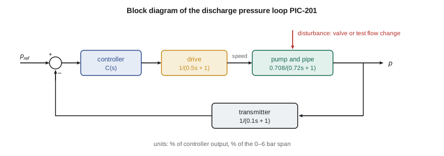
For a proportional controller, \(C(s) = K_c\), the forward path is \(G = K_c \times 0.708/((0.5s + 1)(0.72s + 1))\) and the feedback path is \(H = 1/(0.1s + 1)\). Applying the feedback rule and clearing fractions gives the closed-loop transfer function from setpoint to true pressure:

For \(K_c = 4\), the program multiplies out the polynomials to get a denominator of \(0.036s^3 + 0.482s^2 + 1.32s + 3.832\). Its roots, the closed-loop poles, are at −10.9 and \(-1.23 \pm 2.87j\): the feedback has pulled the two slow real poles together and off the real axis into a complex pair, so the closed loop will oscillate slightly as it settles. The DC gain is \(2.832/3.832 = 0.739\): with proportional control alone, the pressure settles 26 percent short of a setpoint change. Lesson 9 explains why and how to remove the error.

A feature of the closed-loop transfer function deserves attention. The transmitter's lag appears as a zero in the numerator, \(0.1s + 1\), because the transfer function is to the true pressure, not to the measured one. Had Owen asked for the transfer function to the measured pressure, the zero would vanish. The choice of output matters, and a design report should say which is meant.

# Block diagram algebra for the discharge pressure loop, and a state-space model of the drive train
import math, cmath
def pmul(a, b):                       # polynomial product, coefficients highest power first
    r = [0.0]*(len(a) + len(b) - 1)
    for i, x in enumerate(a):
        for j, y in enumerate(b): r[i + j] += x*y
    return r
def padd(a, b):
    n = max(len(a), len(b)); a = [0.0]*(n - len(a)) + a; b = [0.0]*(n - len(b)) + b
    return [x + y for x, y in zip(a, b)]
def roots(p):                         # Durand-Kerner iteration for all roots of a polynomial
    p = [c/p[0] for c in p]; n = len(p) - 1
    z = [complex(0.4, 0.9)**k for k in range(n)]
    for _ in range(500):
        z = [zi - sum(c*zi**(n - k) for k, c in enumerate(p)) / math.prod(zi - zj for j, zj in enumerate(z) if j != i)
             for i, zi in enumerate(z)]
    return sorted(z, key=lambda w: (round(w.real, 6), w.imag))
fmt = lambda p: " + ".join(f"{c:.4g} s^{len(p)-1-i}" if len(p)-1-i > 1 else (f"{c:.4g} s" if len(p)-1-i == 1 else f"{c:.4g}") for i, c in enumerate(p))

# Forward path: controller Kc, drive lag 1/(0.5s+1), pump-and-pipe 0.708/(0.72s+1); feedback: transmitter 1/(0.1s+1)
Kc = 4.0
num_G = [0.708 * Kc]; den_G = pmul([0.5, 1.0], [0.72, 1.0]); num_H = [1.0]; den_H = [0.1, 1.0]
# Closed loop T = G/(1 + G H) = num_G den_H / (den_G den_H + num_G num_H)
num_T = pmul(num_G, den_H); den_T = padd(pmul(den_G, den_H), pmul(num_G, num_H))
print("Closed loop P(s)/Pref(s) =")
print("   numerator:  ", fmt(num_T)); print("   denominator:", fmt(den_T))
print(f"   DC gain {num_T[-1]/den_T[-1]:.3f}: a steady error of {100*(1 - num_T[-1]/den_T[-1]):.0f} % of a setpoint step")
print("   closed-loop poles:", ", ".join(f"{z.real:.2f}{z.imag:+.2f}j" for z in roots(den_T)))

# State-space model of motor, flexible coupling and pump: x = [motor speed, pump speed, coupling twist]
Jm, Jp, kt, bp = 0.090, 0.060, 6.0e3, 0.648
A = [
    [0.0, 0.0, -kt/Jm],
    [0.0, -bp/Jp, kt/Jp],
    [1.0, -1.0, 0.0],
]
B = [1/Jm, 0.0, 0.0]               # input: motor torque
C = [0.0, 0.0, kt]                 # output: torque measured by the coupling transducer
# Characteristic polynomial det(sI - A) by the Faddeev-LeVerrier algorithm
def charpoly(A):
    n = len(A); I = [ [float(i == j) for j in range(n)] for i in range(n)]
    M = [row[:] for row in I]; c = [1.0]
    for k in range(1, n + 1):
        AM = [ [sum(A[i][l]*M[l][j] for l in range(n)) for j in range(n)] for i in range(n)]
        ck = -sum(AM[i][i] for i in range(n)) / k; c.append(ck)
        M = [ [AM[i][j] + ck*I[i][j] for j in range(n)] for i in range(n)]
    return c
cp = charpoly(A)
print("\nDrive train det(sI - A) =", fmt(cp))
for z in roots(cp):
    if abs(z.imag) > 1e-6: print(f"   pole {z.real:.2f} {z.imag:+.1f}j rad/s -> torsional mode at {abs(z)/2/math.pi:.1f} Hz, zeta {-z.real/abs(z):.5f}")
    else: print(f"   pole {z.real:.2f} rad/s -> rigid-body speed mode, time constant {(-1/z.real if z.real else float('inf')):.2f} s")

# Simulate a 10 N m motor torque step (RK4) and record the peak transducer torque
def f(x, u): return [sum(A[i][j]*x[j] for j in range(3)) + B[i]*u for i in range(3)]
x, dt, Tpk = [0.0, 0.0, 0.0], 2e-5, 0.0
for n in range(int(0.2/dt)):
    k1 = f(x, 10.0); k2 = f([a + dt/2*b for a, b in zip(x, k1)], 10.0)
    k3 = f([a + dt/2*b for a, b in zip(x, k2)], 10.0); k4 = f([a + dt*b for a, b in zip(x, k3)], 10.0)
    x = [a + dt/6*(p + 2*q + 2*r + s) for a, p, q, r, s in zip(x, k1, k2, k3, k4)]
    Tpk = max(Tpk, kt*x[2])
print(f"Peak coupling torque after a 10 N m motor step: {Tpk:.2f} N m (rigid-body share {10*Jp/(Jm+Jp):.1f} N m)")

Closed loop P(s)/Pref(s) =
   numerator:   0.2832 s + 2.832
   denominator: 0.036 s^3 + 0.482 s^2 + 1.32 s + 3.832
   DC gain 0.739: a steady error of 26 % of a setpoint step
   closed-loop poles: -10.92+0.00j, -1.23-2.87j, -1.23+2.87j

Drive train det(sI - A) = 1 s^3 + 10.8 s^2 + 1.667e+05 s + 7.2e+05
   pole -4.32 rad/s -> rigid-body speed mode, time constant 0.23 s
   pole -3.24 -408.2j rad/s -> torsional mode at 65.0 Hz, zeta 0.00794
   pole -3.24 +408.2j rad/s -> torsional mode at 65.0 Hz, zeta 0.00794
Peak coupling torque after a 10 N m motor step: 9.53 N m (rigid-body share 4.0 N m)

State variables

The state of a system is the smallest set of variables that, together with the inputs from time zero on, determines its future completely. For a lumped physical system the state variables are naturally the quantities that describe its energy stores: the level in each tank, the temperature of each thermal mass, the velocity of each mass and the deflection of each spring. The number of state variables equals the order of the system. Writing one first-order equation for each and collecting them in matrix form gives the state-space model:

Here x is the state vector, u the input vector, y the output vector, and A, B, C and D are matrices of constant coefficients for a linear time-invariant system. A describes how the states influence each other, B how the inputs drive them, C which combinations are measured and D any direct path from input to output, which is zero for most physical plants.

A state model of the drive train

The two-inertia drive train of Lesson 2 has three energy stores: the kinetic energy of each rotor and the strain energy of the coupling. Choosing the state as motor speed \(\omega_m\), pump speed \(\omega_p\) and coupling twist \(\theta = \theta_m - \theta_p\), with motor torque as the input and the torque measured by the transducer as the output, the equations of Lesson 2 become

The eigenvalues of A are the poles of the system. They are the roots of the characteristic polynomial \(\det(sI - A)\), which the program computes by the Faddeev-LeVerrier algorithm, a simple recursion that needs only matrix products and traces. The result is \(s^3 + 10.8s^2 + 166{,}700s + 720{,}000\), with one real pole at −4.32 rad/s and a complex pair at \(-3.24 \pm 408j\) rad/s. The real pole is the rigid-body speed mode: with no motor slip characteristic in the model (the drive supplies torque directly), the only damping is the pump load, and the train settles with a time constant of 0.23 s. The complex pair is the 65 Hz torsional mode of Lesson 2, with a damping ratio of only 0.008, because the model contains no damping in the coupling itself.

The simulation shows what happens when the motor torque steps by 10 N·m. The coupling torque rings at 65 Hz and peaks at 9.5 N·m within 0.2 s, more than twice the 4.0 N·m share it would carry if the train were rigid at the instant of the step. The ringing is real: torque transducers on test stands often show it during fast speed changes, and it is one reason Gilles leaves the drive's ramp at 5 s.

From state space to transfer function

Taking Laplace transforms of the state equations with zero initial conditions gives \(sX = AX + BU\), so \(X = (sI - A)^{-1}BU\), and the transfer function matrix is

Its denominator is \(\det(sI - A)\), which confirms that the eigenvalues of A are the poles. The reverse conversion is not unique: any transfer function has infinitely many state-space realizations, because the state variables can be chosen in many ways. Standard forms such as the controllable canonical form, in which the coefficients of the denominator appear in the last row of A, are convenient for simulation. Owen's simulations of the pressure loop use the physically meaningful form instead, one state per lag, so that each state can be compared with a measurement during commissioning.

Why both views matter

Block diagrams make the structure of a control system visible, and they are the natural language for discussing where a disturbance enters, where a sensor sits and what a controller acts on. Transfer functions make single-loop design quick. State-space models are better whenever a system has several inputs and outputs, as TL-3 does once level, pressure, flow and temperature are all controlled together; when initial conditions matter; or when nonlinear effects such as saturation are simulated. Modern controller design methods, such as state feedback and observers, are built entirely in state space, and MEC-450 and the mechatronics course build on them. For the single-loop designs of this course, Owen uses transfer functions for design and state-space simulation to check.