
MEC-390 · Lesson 5 of 12 · 23 min
Laplace transforms and transfer functions
By the end of the fourth week Owen has differential equations for every part of TL-3, and Lucie asks him to put them in a form a control engineer can work with. Differential equations are the truth, but they are awkward to combine: connecting the drive, the pump and the transmitter means substituting one equation into another, and adding a controller means doing it again. The Laplace transform turns linear differential equations into algebra, so that each part of the loop becomes a single expression, its transfer function, and connecting parts becomes multiplication. Almost every tool in the rest of the course, from block diagrams to root locus and Bode plots, rests on this step.
The Laplace transform
The Laplace transform of a function f(t), defined for t ≥ 0, is
where s is a complex variable. The integral converts a function of time into a function of s. For engineering work, nobody evaluates the integral each time; a short table of transforms and a few properties are enough. The most important property is the derivative rule: the transform of a derivative is s times the transform of the function, less its initial value,
Differentiation becomes multiplication by s and integration becomes division by s. With zero initial conditions, which is the usual assumption when working with deviation variables about a steady operating point, the initial-value terms vanish and a differential equation becomes an algebraic equation in s.
| f(t), t ≥ 0 | F(s) | Where it appears |
|---|---|---|
| unit impulse δ(t) | 1 | a sudden blow; the hammer of a bump test |
| unit step u(t) | 1/s | a setpoint change or a valve opened suddenly |
| ramp t | 1/s² | a drive following its acceleration ramp |
| e^(−at) | 1/(s + a) | first-order decay |
| sin ωt | ω/(s² + ω²) | harmonic input or response |
| e^(−at) sin ωt | ω/((s + a)² + ω²) | damped oscillation |
| f(t − T) u(t − T) | e^(−sT) F(s) | a pure time delay |
Transfer functions
The transfer function of a linear time-invariant system is the ratio of the Laplace transform of its output to that of its input, with all initial conditions zero. For the linearized suction tank of Lesson 1, \(\tau\,d\Delta h/dt + \Delta h = R\,\Delta q_{in}\) transforms to \((\tau s + 1)H(s) = RQ_{in}(s)\), so
The bearing frame of Lesson 3 has exactly the same form, \(G(s) = 0.22/(2966s + 1)\) K/W, which is why every first-order system behaves alike. The transfer function contains everything about the system's linear input-output behavior and nothing about its internal states or initial conditions. The numerator gives the zeros, values of s that make G zero; the denominator gives the poles, values of s that make G infinite. The polynomial in the denominator, set to zero, is the characteristic equation, and its roots govern the free response.
For the valve stem of Lesson 2, \(m\ddot x + c\dot x + kx = F\) transforms to \((ms^2 + cs + k)X(s) = F(s)\), giving
and for the hydraulic actuator of Lesson 4, an integrator, \(G_{act}(s) = Y(s)/U(s) = K_q/(A_cs) = 20.4/s\) mm per V·s. The three types, first-order lag, second-order system and integrator, are the building blocks from which almost every plant in this course is made.
Poles and the free response
The location of each pole in the complex s-plane tells what kind of motion it contributes to the response. A real pole at \(s = -a\) contributes a term \(e^{-at}\), decaying with time constant 1/a. A pair of complex poles at \(s = -\sigma \pm j\omega_d\) contributes a decaying oscillation \(e^{-\sigma t}\sin(\omega_d t + \phi)\). Poles in the left half of the plane give decaying terms; poles in the right half give growing ones, and the system is unstable. Poles far to the left decay quickly, so the poles closest to the imaginary axis, the dominant poles, govern the response that is seen.
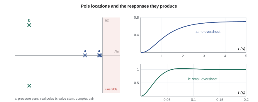
The pressure process modeled in Lesson 4 is a gain of 0.708 with three lags in series. Its transfer function is the product of the three first-order transfer functions:
with poles at s = −2.0, −1.39 and −10 rad/s, all real and negative. The two slow poles dominate; the transmitter's pole at −10 decays five times faster and hardly shows. The valve stem's poles are at \(-41.7 \pm 40.0j\) rad/s, a complex pair with a damping ratio of 0.72, and they are so far to the left that the stem's dynamics are over long before the pressure plant has moved.
Inverse transforms by partial fractions
To get a time response from a transfer function, multiply by the transform of the input and invert. The usual method is to expand the result into partial fractions, each of which appears in the table. For a unit step into the pressure plant, \(Y(s) = G_p(s)/s\), and with distinct real poles the expansion is
Each coefficient is found by the cover-up rule: multiply by the factor containing that pole and evaluate at the pole. The residue at s = 0 is simply the steady-state gain, \(A_0 = G_p(0) = 0.708\). The program computes all four and inverts term by term, giving
# Transfer functions of the TL-3 models, inverse Laplace transforms by partial fractions, and a check by simulation
import math, cmath
# Tank: H(s)/Qin(s) = R/(tau s + 1), R = 120 s/m^2, tau = 480 s.  Bearing frame: T(s)/Q(s) = 0.22/(2966 s + 1)
for name, K, tau, step, unit in (("tank level", 120.0, 480.0, 0.005, "m"), ("bearing frame", 0.22, 2966.0, 180.0, "K")):
    print(f"{name}: G(s) = {K}/({tau:.0f} s + 1); step of {step} gives final value K*step = {K*step:.3f} {unit}"
          f" (final value theorem: lim s->0 of s G(s) step/s)")

# Third-order pressure plant: G(s) = 0.708 / ((0.5 s + 1)(0.72 s + 1)(0.1 s + 1))
K = 0.708; taus = [0.5, 0.72, 0.1]
poles = [-1/t for t in taus]
gain = K / math.prod(taus)                       # G(s) = gain / ((s - p1)(s - p2)(s - p3))
print(f"\nPressure plant poles: {', '.join(f'{p:.3f}' for p in poles)} rad/s; high-frequency gain {gain:.2f}")
# Unit step: Y(s) = G(s)/s.  Residue at s = 0 is G(0) = K; residue at each pole p_i is gain/(p_i prod(p_i - p_j))
res = []
for i, p in enumerate(poles):
    den = p * math.prod(p - q for j, q in enumerate(poles) if j != i)
    res.append(gain / den)
print("Partial fractions: y(t) = " + f"{K:.3f}" + "".join(f" {'+' if r >= 0 else '-'} {abs(r):.3f} e^({p:.3f} t)" for r, p in zip(res, poles)))
y = lambda t: K + sum(r*math.exp(p*t) for r, p in zip(res, poles))

# Check against a direct simulation of the three lags in series (RK4)
def deriv(x, u):
    d = []; inp = u
    for xi, t in zip(x, taus): d.append((inp - xi)/t); inp = xi
    return d
x, dt, sim = [0.0, 0.0, 0.0], 0.001, {}
for n in range(5001):
    t = n*dt
    if n % 500 == 0: sim[round(t, 2)] = K*x[2]
    k1 = deriv(x, 1); k2 = deriv([a + dt/2*b for a, b in zip(x, k1)], 1)
    k3 = deriv([a + dt/2*b for a, b in zip(x, k2)], 1); k4 = deriv([a + dt*b for a, b in zip(x, k3)], 1)
    x = [a + dt/6*(p + 2*q + 2*r + s) for a, p, q, r, s in zip(x, k1, k2, k3, k4)]
print("  t (s)  partial fractions  simulation")
for t, v in sim.items(): print(f"  {t:4.1f}      {y(t) + 1e-12:7.4f}          {v:7.4f}")

# Valve stem, second order: X(s)/F(s) = 1/(m s^2 + c s + k); complex poles
m, c, k = 18.0, 1500.0, 60e3
disc = cmath.sqrt(c*c - 4*m*k)
s1, s2 = (-c + disc)/(2*m), (-c - disc)/(2*m)
print(f"\nValve stem poles: {s1.real:.1f} +/- {abs(s1.imag):.1f}j rad/s; damped frequency {abs(s1.imag)/2/math.pi:.2f} Hz")tank level: G(s) = 120.0/(480 s + 1); step of 0.005 gives final value K*step = 0.600 m (final value theorem: lim s->0 of s G(s) step/s) bearing frame: G(s) = 0.22/(2966 s + 1); step of 180.0 gives final value K*step = 39.600 K (final value theorem: lim s->0 of s G(s) step/s) Pressure plant poles: -2.000, -1.389, -10.000 rad/s; high-frequency gain 19.67 Partial fractions: y(t) = 0.708 + 2.011 e^(-2.000 t) - 2.691 e^(-1.389 t) - 0.029 e^(-10.000 t) t (s) partial fractions simulation 0.0 0.0000 0.0000 0.5 0.1041 0.1041 1.0 0.3092 0.3092 1.5 0.4731 0.4731 2.0 0.5775 0.5775 2.5 0.6380 0.6380 3.0 0.6713 0.6713 3.5 0.6890 0.6890 4.0 0.6983 0.6983 4.5 0.7031 0.7031 5.0 0.7055 0.7055 Valve stem poles: -41.7 +/- 40.0j rad/s; damped frequency 6.36 Hz
The partial-fraction result and the Runge-Kutta simulation agree to four decimal places at every time printed. Two points are worth noticing. The coefficient of the fast transmitter pole, 0.029, is tiny: its term barely affects the response, confirming that the pole contributes little. And the two large coefficients of opposite sign on the slow poles nearly cancel at t = 0, producing the S-shaped start typical of systems with several lags. The response reaches 0.31 of a unit after one second and 0.70 after four.
Final and initial value theorems
Two theorems give limiting values without inverting. The final value theorem states that if the limit exists, which requires all poles of sF(s) to lie in the left half-plane,
For a step of size \(q_s\) into any system, \(sG(s)q_s/s = G(s)q_s\), so the final value is \(G(0)q_s\), the DC gain times the step. A 0.005 m³/s inflow step raises the tank level by \(120 \times 0.005 = 0.6\) m; a 180 W heat step raises the bearing frame by 39.6 K. The theorem must be used with care: applied to an integrator, \(G(s) = 20.4/s\), it gives an infinite final value for a step input, correctly predicting that the actuator runs to its stop. Applied to an unstable system it gives a finite number that is meaningless, which is why the stability condition comes first.
Worked problem
Response of the bearing frame to a cooler failure
The bearing frame runs at a steady 42.6 °C with the oil cooler on (R = 0.12 K/W, τ = 27 min). The cooling water fails, and the resistance returns to 0.22 K/W. Treating the change as a step in steady rise from 21.6 to 39.6 K that develops with the new time constant of 49 min, find the temperature after 30 minutes and the final temperature.
Show solution
- The deviation from the old steady state is a step of 18.0 K into \(G(s) = 1/(2966s + 1)\).
- Time response \(\Delta T(t) = 18.0(1 - e^{-t/2966})\).
- At 30 min (1,800 s), \(\Delta T = 18.0(1 - e^{-0.607}) = 18.0 \times 0.455 = 8.2\) K, so T ≈ 50.8 °C.
- Final value from the theorem: \(42.6 + 18.0 = 60.6\) °C.
Answer: A high-temperature alarm at 55 °C would sound about 58 minutes after the failure, which gives operators ample time to stop the test.
Transfer functions with zeros and delays
Some processes have zeros, which shape the response without changing the poles. A zero at \(s = -z\) in the left half-plane speeds up the response and can cause overshoot even in a system with real poles; a zero in the right half-plane makes the response start in the wrong direction, as happens with the level in a boiler drum when feedwater is added. TL-3 has none of note, but Lesson 10 adds a zero deliberately with a PI controller.
Pure time delays are common in fluid and thermal systems. When the oil temperature sensor sits in the return line a few meters from the bearing, the oil takes time to travel there, and the measurement repeats the bearing temperature T seconds late. The delay's transfer function is \(e^{-sT}\), which is not a ratio of polynomials. It has magnitude one at every frequency but adds phase lag that grows without limit, and Lesson 11 shows that it is the single most damaging element a feedback loop can contain. For analysis, a Padé approximation such as \(e^{-sT} \approx (1 - sT/2)/(1 + sT/2)\) replaces it with a right-half-plane zero and a pole.
Common mistakes
MistakeForgetting that transfer functions assume zero initial conditions.
InsteadWork in deviation variables about a steady state, where initial deviations are zero.
MistakeApplying the final value theorem to an unstable or integrating system without checking.
InsteadCheck that all poles of sF(s) are in the left half-plane first.
MistakeReading the step response's speed from the fastest pole.
InsteadThe dominant poles, closest to the imaginary axis, set the visible response.
MistakeDropping a small residue's pole and its gain together.
InsteadWhen simplifying, keep the DC gain unchanged.
MistakeTreating a time delay as a lag.
InsteadA delay shifts the whole response and adds unlimited phase lag; a lag does not.
Summary and key terms
- The Laplace transform turns derivatives into multiplication by s and integrals into division by s.
- A transfer function is output over input in s, with zero initial conditions; its poles and zeros characterize the system.
- First-order lag, second-order system and integrator are the basic building blocks.
- The pressure plant 0.708/((0.5s + 1)(0.72s + 1)(0.1s + 1)) has poles at −2.0, −1.39 and −10 rad/s.
- Partial fractions invert responses term by term; the step response is 0.708 + 2.011e^(−2t) − 2.691e^(−1.389t) − 0.029e^(−10t).
- The final value theorem gives the steady response G(0) × step when all poles of sF(s) are stable.
- Laplace transform
- The integral transform that converts a function of time into a function of the complex variable s.
- Transfer function
- The ratio of output to input transforms of a linear system with zero initial conditions.
- Pole
- A root of the denominator of a transfer function.
- Zero
- A root of the numerator of a transfer function.
- Characteristic equation
- The denominator of a transfer function set to zero.
- DC gain
- The steady-state gain G(0) of a stable system.
- Dominant poles
- The poles closest to the imaginary axis, which govern the visible response.
- Partial fractions
- Expansion of a rational function into simple terms that can be inverted from a table.
- Final value theorem
- The rule that the final value of f(t) equals the limit of sF(s) as s tends to zero.
- Padé approximation
- A rational function used to approximate a time delay.
Practice problems
Work each problem on paper first, then reveal the answer to check.
Write the transfer function of a tank with A = 2.0 m² and R = 150 s/m².
Show answer
150/(300s + 1).
Where are the poles of 4/(s² + 4s + 13)?
Show answer
s = −2 ± 3j.
Find the final value of the step response of 5/((s + 1)(s + 5)).
Show answer
G(0) = 5/5 = 1.
Find the partial fraction coefficients of 1/(s(s + 2)).
Show answer
1/(s(s + 2)) = 0.5/s − 0.5/(s + 2).
In the program, change the transmitter lag from 0.1 to 0.3 s. What happens to its residue?
Show answer
It grows from −0.029 to about −0.76, since the pole at −3.33 is closer to the others and its term becomes visible.
What is the transfer function of a 3 s pure delay?
Show answer
e^(−3s).
Lesson quiz · 5 questions
Score 60% or more to complete this lesson.
Create a free account to save your progress, take quizzes and earn a certificate.