Fluid and thermal systems

Most of TL-3 is water moving through pipes and heat moving through metal, so Owen's next models are fluid and thermal. Mechanical engineers sometimes treat these as a separate subject, but Lucie insists on the opposite view. The same three kinds of element appear in every energy domain: something that stores energy in one form, something that stores it in another, and something that dissipates it. Once Owen can see a tank as a capacitor and a long pipe as an inertia, the methods of Lesson 2 carry straight over.

Effort, flow and power

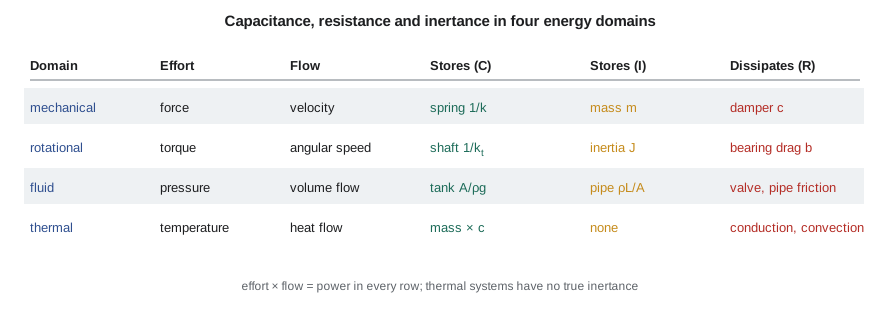
In each domain, one variable can be thought of as an effort, which drives motion, and another as a flow, which is the resulting motion. Their product is power. In translational mechanics, force times velocity is power; in rotation, torque times angular speed; in a liquid system, pressure times volumetric flow rate; in an electrical circuit, voltage times current. Thermal systems are the exception: temperature and heat flow rate are used as effort and flow because they are what engineers measure, but their product is not a power. The analogy is still useful as long as that difference is remembered.

Fluid capacitance

A fluid capacitance stores fluid and relates the volume stored to the pressure or head. For an open tank with vertical sides, the stored volume is \(V = Ah\), and the pressure at the bottom is \(p = \rho gh\). The capacitance, defined as the change in volume per change in effort, is

The suction tank T-101 has C = 4.0 m² in head form or about \(409 \times 10^{-6}\) m³/Pa in pressure form. Which form to use is a matter of convenience; Owen works in head for the water circuit because pump curves are drawn in head. A tank with sloping sides has a capacitance that varies with level, which makes it nonlinear even when the outflow is linear.

Closed vessels store fluid by compressing it. For a liquid of bulk modulus β in a rigid container of volume V, a change in pressure dp changes the stored mass by an amount equivalent to a volume \(dV = (V/\beta)dp\), so \(C = V/\beta\). Water's bulk modulus is about 2.2 GPa and hydraulic oil's is similar, but hoses and trapped air reduce the effective value considerably. For the actuator of FV-301, with about 0.9 liter of oil trapped in the hoses and cylinder and an effective bulk modulus of 1.4 GPa including hose compliance, the capacitance is only \(6.4 \times 10^{-13}\) m³/Pa: forcing one extra cubic centimeter of oil into the circuit raises its pressure by about 16 bar. That stiffness is why hydraulic actuators can position heavy loads precisely, and why a small leak or a little entrained air changes their behavior so much.

Gas is far more compressible. For an ideal gas held at constant temperature in a receiver of volume V, the stored mass is \(m = pV/(RT)\), so the pneumatic capacitance is \(C = dm/dp = V/(RT)\). The test bay's 0.5 m³ instrument-air receiver has \(C = 5.95 \times 10^{-6}\) kg/Pa. If the compressor stops while the instruments and valve positioners keep drawing 12 g/s, the receiver pressure falls about 1.2 bar per minute, which tells Gilles how long the bay can run on stored air and sets the low-pressure alarm. If the compression is fast enough to be adiabatic rather than isothermal, the capacitance is smaller by the ratio of specific heats, 1.4 for air.

Fluid resistance

Fluid resistance relates the flow through a restriction to the pressure or head difference across it. For laminar flow in a long capillary, the relationship is linear, as the Hagen-Poiseuille law shows. In nearly every industrial water system the flow is turbulent, and the head loss across a valve or along a pipe varies with the square of the flow, \(\Delta H = aq^2\). As Lesson 1 showed, such an element is linearized about its operating flow \(q_0\), giving a resistance

In the discharge circuit of TL-3, the throttling valve and the pipe together lose about 9 m of head at the design flow of 0.025 m³/s, so their linearized resistance is \(2 \times 9/0.025 = 720\) s/m². The factor of 2 is easy to forget, and forgetting it halves the predicted time constants of every flow loop.

Fluid inertance

Water in a pipe has mass, and changing its velocity takes a pressure difference. For a slug of liquid of length L in a pipe of area \(A_p\), Newton's second law gives \(\Delta p\,A_p = \rho LA_p\,dv/dt\). Writing the velocity in terms of volume flow, \(v = q/A_p\),

The inertance I is the fluid counterpart of mass, and it matters most in long, small pipes. The 12 m suction line of 150 mm diameter has I = 69 s²/m² in head form; the 40 m discharge line of 100 mm diameter has 519 s²/m². Combining the discharge line's inertance with the loop's resistance gives a first-order flow equation, \(I\,dq/dt + Rq = \Delta H\), whose time constant is \(I/R = 519/720 = 0.72\) s. When the drive changes speed, the flow takes most of a second to build up to its new value. That 0.72 s lag will appear in the pressure loop model of Lesson 6.

Inertance also explains water hammer. If a valve closes in a time much shorter than the pipe's dynamics, the pressure rise \(I\,dq/dt\) becomes enormous; a full treatment needs the compressibility of the water and the elasticity of the pipe, which turn the lumped model into a traveling wave, as MEC-370 discussed. Farah's specification limits FV-301 to a closing time of at least 5 s for this reason, and Owen's model will respect that limit as a rate constraint on the actuator.

# Fluid and thermal elements on the TL-3 loop: capacitance, resistance and inertance, and the bearing temperature model
import math
rho, g = 998.0, 9.81
# Liquid capacitance of the suction tank (level form and pressure form)
A = 4.0
print(f"Tank T-101: C = {A:.1f} m^2 (level per volume), or {A/(rho*g)*1e6:.0f} x 10^-6 m^3/Pa in pressure form")

# Inertance of the water in a pipe: head form I = L/(g A), pressure form rho L / A
def inertance(L, D):
    Ap = math.pi * D**2 / 4
    return L / (g * Ap), rho * L / Ap
for name, L, D in (("suction line", 12.0, 0.150), ("discharge line", 40.0, 0.100)):
    Ih, Ip = inertance(L, D)
    print(f"{name:15s} L = {L:4.0f} m, D = {D*1000:.0f} mm: I = {Ih:6.1f} s^2/m^2 (head), {Ip/1e6:5.2f} x 10^6 kg/m^4 (pressure)")

# Flow build-up when the throttling valve opens: inertance against linearized loop resistance
Ih, _ = inertance(40.0, 0.100)
q0, H_loss = 0.025, 9.0            # flow (m^3/s) and head lost in the valve and pipe at that flow (m)
R_lin = 2 * H_loss / q0            # for losses proportional to q^2
print(f"Loop resistance {R_lin:.0f} s/m^2, flow time constant I/R = {Ih/R_lin:.2f} s")

# Hydraulic capacitance of oil in the actuator hoses and cylinder: C = V / beta
beta, V = 1.4e9, 0.9e-3            # effective bulk modulus (Pa) with hose compliance, trapped volume (m^3)
print(f"Oil capacitance V/beta = {V/beta:.2e} m^3/Pa: 1 cm^3 of extra oil raises pressure by {1e-6/(V/beta)/1e5:.1f} bar")

# Pneumatic capacitance of the instrument air receiver (isothermal): C = V/(R T)
Vr, Tair, Rg = 0.50, 293.0, 287.0
Cp = Vr / (Rg * Tair)              # kg/Pa
mdot = 0.012                       # air demand with the compressor stopped, kg/s
print(f"Air receiver C = {Cp*1e6:.2f} x 10^-6 kg/Pa; pressure falls {mdot/Cp/1e5*60:.2f} bar per minute at {mdot*1000:.0f} g/s")

# Thermal model of the bearing frame: C dT/dt = Q - (T - Ta)/R
Cth = 25.0*460 + 1.2*0.87*1900    # metal plus oil, J/K
Rth, Q, Ta = 0.22, 180.0, 21.0     # K/W, bearing friction heat (W), ambient (deg C)
tau = Rth * Cth
print(f"\nBearing frame: C = {Cth/1000:.1f} kJ/K, R = {Rth} K/W, tau = {tau:.0f} s ({tau/60:.0f} min)")
print(f"Steady rise {Q*Rth:.1f} K, so the frame settles near {Ta + Q*Rth:.1f} deg C")
logged = [(0, 21.0), (30, 39.5), (60, 49.8), (90, 55.0), (120, 57.6), (180, 59.9), (240, 60.4)]
print("  t (min)  model (deg C)  logged (deg C)")
for tm, Tl in logged:
    Tm = Ta + Q*Rth*(1 - math.exp(-tm*60/tau))
    print(f"  {tm:5d}     {Tm:6.1f}         {Tl:6.1f}")
# With the oil cooler in service the resistance to ambient falls to 0.12 K/W
print(f"With the cooler on (R = 0.12 K/W): rise {Q*0.12:.1f} K, tau {0.12*Cth/60:.0f} min")

Tank T-101: C = 4.0 m^2 (level per volume), or 409 x 10^-6 m^3/Pa in pressure form
suction line    L =   12 m, D = 150 mm: I =   69.2 s^2/m^2 (head),  0.68 x 10^6 kg/m^4 (pressure)
discharge line  L =   40 m, D = 100 mm: I =  519.2 s^2/m^2 (head),  5.08 x 10^6 kg/m^4 (pressure)
Loop resistance 720 s/m^2, flow time constant I/R = 0.72 s
Oil capacitance V/beta = 6.43e-13 m^3/Pa: 1 cm^3 of extra oil raises pressure by 15.6 bar
Air receiver C = 5.95 x 10^-6 kg/Pa; pressure falls 1.21 bar per minute at 12 g/s

Bearing frame: C = 13.5 kJ/K, R = 0.22 K/W, tau = 2966 s (49 min)
Steady rise 39.6 K, so the frame settles near 60.6 deg C
  t (min)  model (deg C)  logged (deg C)
      0       21.0           21.0
     30       39.0           39.5
     60       48.8           49.8
     90       54.2           55.0
    120       57.1           57.6
    180       59.6           59.9
    240       60.3           60.4
With the cooler on (R = 0.12 K/W): rise 21.6 K, tau 27 min

Thermal capacitance and resistance

A body of mass m and specific heat c stores thermal energy; its thermal capacitance is \(C = mc\), in J/K. Heat flows through thermal resistances: by conduction through a wall of thickness L, area A and conductivity k, \(R = L/(kA)\); by convection from a surface of area A with coefficient h, \(R = 1/(hA)\). A body that is small or conductive enough to have a nearly uniform temperature, the condition MEC-340 expressed as a Biot number well below 0.1, can be modeled as a single lump. Its energy balance is

which is first order, with time constant \(\tau = RC\) and steady temperature rise \(\dot Q_{in}R\). Thermal systems have no true inertance, since heat does not have momentum, so a network of thermal lumps and resistances can never oscillate on its own. Its response is always a sum of decaying exponentials.

The bearing frame

The TP-80's bearing frame, about 25 kg of cast iron, holds 1.2 liters of oil. Its thermal capacitance is \(25 \times 460 + 1.2 \times 0.87 \times 1{,}900 \approx 13.5\) kJ/K. The two ball bearings and the oil churning generate about 180 W at full speed. The resistance from the frame to the surrounding air, through natural convection and radiation from the fins and through conduction into the baseplate, is about 0.22 K/W. The model predicts a steady rise of 39.6 K, so the frame settles near 61 °C in a 21 °C test bay, with a time constant of 2,966 s, or 49 minutes.

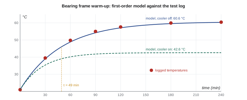
Lucie pulls a test record from the old stand, which logged the bearing temperature of a TP-80 during a four-hour endurance run. The model tracks the log within about 1 °C throughout. The logged values run slightly ahead of the model in the first hour, which suggests the true time constant is a little shorter; Lesson 7 shows how to extract it from the log. Either way, the conclusion for control design is clear. The bearing temperature is a slow, first-order process with a time constant of the better part of an hour. A temperature controller acting on the oil cooler will need patience, and tests cannot start their readings until the bearings have warmed for two hours or more.

With the oil cooler valve open, cooling water carries heat away and the resistance to ambient falls to about 0.12 K/W. The steady rise drops to 21.6 K and the time constant to 27 minutes. Because opening the cooler changes R, it changes both the gain and the time constant of the process: a controller tuned with the cooler closed will see a different plant with it open. Owen notes this nonlinearity for Lesson 12.

Interacting and non-interacting systems

When two stores are connected in series, the way they are connected matters. If the first tank discharges freely into the second, the second tank's level cannot affect the first tank's outflow, and the two first-order systems are non-interacting: the overall response is simply the product of two first-order responses. If the tanks are joined at the bottom by a pipe, the flow between them depends on the difference in their levels, so each tank affects the other. Such interacting systems have the same order, but their time constants are spread further apart than the individual RC products would suggest. The same distinction applies to thermal lumps in contact and to masses joined by springs. Recognizing which case applies saves effort in Lesson 6, where state-space models handle the interacting case naturally.