
MEC-390 · Lesson 11 of 12 · 22 min
Frequency response and Bode plots
Lucie has spent her career looking at vibration spectra, and she thinks about systems in terms of frequency. When Owen shows her the root locus of the PI pressure loop, she asks a question it cannot answer directly: what happens if the oil temperature sensor, mounted a few meters down the return line, adds a fraction of a second of pure delay? Delays do not fit the root locus rules, because \(e^{-sT}\) is not a ratio of polynomials. The frequency response handles them without difficulty, and it has another advantage that suits a test laboratory: it can be measured. Feed a sine wave into a stable system, wait for the transient to die, and the output is a sine wave of the same frequency, scaled and shifted. Those two numbers at every frequency are the frequency response.
Frequency response
For a stable linear system G(s), a steady sinusoidal input \(u = U\sin\omega t\) produces a steady output
The amplitude ratio is the magnitude of G evaluated at \(s = j\omega\), and the phase shift is its angle. Lucie recognizes this at once as the frequency response function of MEC-380, measured there with a hammer and an accelerometer; for a control loop it is measured with a sine sweep from the controller or computed from the model. For a first-order lag \(1/(\tau s + 1)\), \(|G(j\omega)| = 1/\sqrt{1 + (\omega\tau)^2}\) and \(\angle G = -\arctan\omega\tau\): at low frequencies the output follows the input; at \(\omega = 1/\tau\), the corner frequency, the amplitude has fallen to 0.707 and the phase lags by 45°; at high frequencies the amplitude falls in proportion to 1/ω and the lag approaches 90°.
Bode plots
Hendrik Bode, working on telephone amplifiers in the 1930s and 1940s, introduced the plots that carry his name: magnitude in decibels, \(20\log_{10}|G|\), and phase in degrees, both against frequency on a logarithmic axis. The logarithms turn products into sums, so the Bode plot of a loop made of many blocks is the sum of the plots of the blocks. Each standard factor has a simple straight-line approximation, the asymptotes, that can be drawn by hand.
| Factor | Magnitude asymptote | Phase |
|---|---|---|
| constant K | flat at 20 log K | 0° |
| integrator 1/s | −20 dB/decade, 0 dB at ω = 1 | −90° at all ω |
| lag 1/(τs + 1) | flat, then −20 dB/decade after ω = 1/τ | 0° to −90°, −45° at 1/τ |
| lead (τs + 1) | flat, then +20 dB/decade after ω = 1/τ | 0° to +90° |
| second order, ωₙ, ζ | flat, then −40 dB/decade after ωₙ; peak if ζ < 0.7 | 0° to −180° |
| delay e^(−sT) | 0 dB at all ω | −ωT rad, growing without limit |
The magnitude asymptote of a lag is accurate to within 3 dB, the worst error falling at the corner. The phase changes over about two decades centered on the corner. The time delay is unusual: it leaves the magnitude untouched but adds a phase lag proportional to frequency, so on a logarithmic axis its phase curve falls ever more steeply.
The pressure loop's Bode plot
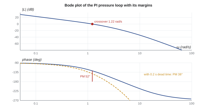
For the PI loop designed in Lesson 10 (\(K_c = 1.46\), \(T_i = 0.72\) s), the loop transfer function contains an integrator, the gain \(1.46 \times 0.708/0.72 = 1.44\) after cancellation, and lags with corners at 2 and 10 rad/s. The magnitude falls at 20 dB/decade from low frequencies, crosses 0 dB at 1.22 rad/s, then steepens to 40 and finally 60 dB/decade beyond the two corners. The phase starts at −90° because of the integrator and falls toward −270° as the lags add their 90° each.
Gain and phase margins
Stability of the closed loop can be read from the open-loop Bode plot. At the gain crossover frequency \(\omega_c\), where \(|L(j\omega)| = 1\), the phase margin is how far the phase is above −180°: \(PM = 180^\circ + \angle L(j\omega_c)\). At the phase crossover frequency \(\omega_{180}\), where the phase is −180°, the gain margin is how far the magnitude is below 0 dB: \(GM = -20\log_{10}|L(j\omega_{180})|\). If both margins are positive, the closed loop is stable (for loops whose open-loop poles are all stable, which covers every loop in this course). The gain margin agrees with the Routh result of Lesson 8; the phase margin is new, and it is the margin that delays consume.
The margins measure robustness. The gain margin says how much the plant's gain may grow before the loop goes unstable; the phase margin says how much extra lag, from a delay, a slow sensor or a neglected dynamic, the loop can tolerate at its crossover frequency. Typical targets are a gain margin of at least 6 dB and a phase margin of 45° to 60°. A phase margin of about 50° to 60° usually gives a step response with modest overshoot, roughly 10 to 20 percent for loops containing an integrator.
# Frequency response of the pressure loop: Bode values, crossover, gain and phase margins, and the effect of dead time
import math, cmath
def L(w, Kc, Ti=None, delay=0.0):
    s = 1j*w
    G = 0.708/((0.5*s + 1)*(0.72*s + 1)*(0.1*s + 1))
    C = Kc*(1 + 1/(Ti*s)) if Ti else Kc
    return C*G*cmath.exp(-s*delay)
def margins(Kc, Ti=None, delay=0.0):
    ws = [10**(k/2000) for k in range(-6000, 4001)]          # 0.001 to 100 rad/s
    wc = wg = None; prev = None
    for w in ws:
        v = L(w, Kc, Ti, delay); mag = abs(v); ph = math.degrees(cmath.phase(v))
        ph_unw = ph if prev is None else prev[1] + ((ph - prev[1] + 180) % 360 - 180)
        if prev and prev[0] >= 1 > mag and wc is None: wc, pm = w, 180 + ph_unw
        if prev and prev[1] > -180 >= ph_unw and wg is None: wg, gm = w, -20*math.log10(mag)
        prev = (mag, ph_unw)
    return wc, pm, wg, gm
print("Bode values of the PI loop (Kc = 1.46, Ti = 0.72 s)")
print("   w (rad/s)   |L| (dB)   phase (deg)")
ph_prev = None
for w in (0.1, 0.3, 1.0, 1.39, 2.0, 3.0, 6.0, 10.0, 30.0):
    v = L(w, 1.46, 0.72); ph = math.degrees(cmath.phase(v))
    if ph > 0: ph -= 360
    print(f"   {w:8.2f}   {20*math.log10(abs(v)):7.1f}    {ph:8.1f}")
print("\n  loop                                crossover (rad/s)  PM (deg)  phase crossover (rad/s)  GM (dB)")
for lab, Kc, Ti, d in (("P, Kc = 4", 4.0, None, 0.0), ("PI, Kc = 1.46, Ti = 0.72 s", 1.46, 0.72, 0.0),
                       ("PI, same, 0.2 s dead time", 1.46, 0.72, 0.2), ("PI, Kc = 3.0, 0.2 s dead time", 3.0, 0.72, 0.2)):
    wc, pm, wg, gm = margins(Kc, Ti, d)
    print(f"  {lab:34s}  {wc:8.2f}           {pm:6.1f}       {wg:8.2f}             {gm:6.1f}")
# Dead time costs phase: 0.2 s at the crossover frequency of the PI loop
wc = margins(1.46, 0.72)[0]
print(f"\nA 0.2 s delay removes {math.degrees(0.2*wc):.1f} deg of phase at w = {wc:.2f} rad/s without changing |L|")Bode values of the PI loop (Kc = 1.46, Ti = 0.72 s)
w (rad/s) |L| (dB) phase (deg)
0.10 23.1 -93.4
0.30 13.5 -100.2
1.00 2.1 -122.3
1.39 -1.5 -132.7
2.00 -6.1 -146.3
3.00 -11.9 -163.0
6.00 -23.8 -192.5
10.00 -34.0 -213.7
30.00 -59.9 -247.8
loop crossover (rad/s) PM (deg) phase crossover (rad/s) GM (dB)
P, Kc = 4 2.19 62.4 6.06 15.4
PI, Kc = 1.46, Ti = 0.72 s 1.22 51.7 4.48 18.5
PI, same, 0.2 s dead time 1.22 37.8 2.36 8.3
PI, Kc = 3.0, 0.2 s dead time 2.03 9.8 2.36 2.1
A 0.2 s delay removes 14.0 deg of phase at w = 1.22 rad/s without changing |L|The program evaluates the loop at many frequencies and finds the crossovers numerically. The PI design has a crossover at 1.22 rad/s, a phase margin of 51.7° and a gain margin of 18.5 dB, comfortably inside the targets. For comparison, the proportional loop at \(K_c = 4\) crosses over faster, at 2.19 rad/s, with a phase margin of 62° and the 15.4 dB gain margin found in Lesson 8; its larger margin does not save it, because it fails the accuracy requirement.
The cost of dead time
Now Lucie's question. Suppose the measurement arrives 0.2 s late, because the transmitter's averaging or a long impulse line delays it. The delay does not change the magnitude, so the crossover stays at 1.22 rad/s, but it removes \(0.2 \times 1.22\) rad, or 14°, of phase there. The program shows the phase margin falling from 51.7° to 37.8°, and the phase crossover moving down from 4.48 to 2.36 rad/s, which cuts the gain margin from 18.5 to 8.3 dB. The loop is still stable but noticeably more oscillatory. Doubling the controller gain to \(K_c = 3.0\) with the delay present would leave a phase margin of under 10° and a gain margin of 2 dB, a loop close to the edge.
The general lesson, which Owen writes at the top of his design notes, is that delay limits how fast any loop can be made. Since a delay of T costs ωT radians at crossover, keeping its cost below, say, 30° requires \(\omega_c < 0.5/T\). A loop with 0.2 s of delay cannot reasonably be given a crossover above about 2.5 rad/s, however clever the controller. Long sensor lines, slow analyzer sampling and transport delays in pipes are therefore design issues, not details.
Worked problem
Delay in the bearing temperature loop
The oil temperature sensor TT-401 sits in the oil return line 2.4 m from the bearing, and the oil flows at about 0.06 m/s. The temperature loop, acting on the cooler valve, is designed for a crossover of 0.004 rad/s. How much phase does the transport delay cost, and does it matter?
Show solution
- Delay \(T = 2.4/0.06 = 40\) s.
- Phase lost at crossover \(= \omega_cT = 0.004 \times 40 = 0.16\) rad = 9.2°.
Answer: About 9° is a modest cost against a target margin of 45° or more, because the thermal process is so slow. The same 40 s delay in the pressure loop, whose crossover is 300 times higher, would make control impossible. Delays matter in proportion to how fast the loop must be.
Bandwidth and the closed-loop frequency response
The closed-loop frequency response \(T(j\omega)\) is close to 1 at low frequencies, where the loop gain is high, and falls away above the crossover. The bandwidth, the frequency at which \(|T|\) has fallen 3 dB below its low-frequency value, is usually close to the crossover frequency, and it is the frequency-domain measure of speed: rise time is roughly \(2/\omega_{BW}\) for well-damped loops. A resonant peak in \(|T|\) corresponds to poorly damped closed-loop poles and to overshoot in the step response; the peak grows as the phase margin shrinks. The sensitivity function \(|S(j\omega)|\) is small below crossover, where disturbances are rejected, and has a peak just above it, where disturbances are amplified; a large peak, typically more than 2, is another sign of an aggressive design.
Nyquist's view
Harry Nyquist, a colleague of Bode, gave the general stability test from which the margins come. Plotting \(L(j\omega)\) in the complex plane as ω runs from zero to infinity traces the Nyquist curve. For a loop whose open-loop poles are all stable, the closed loop is stable if the curve does not encircle the point −1. The gain margin is how far the curve passes from −1 along the negative real axis; the phase margin is the angle, measured where the curve crosses the unit circle, between the curve and the negative real axis. The Nyquist criterion also handles open-loop unstable plants, by counting encirclements, and loops with delays, which simply wind the curve into a spiral. For the loops in this course, the Bode margins carry the same information in a more convenient form.
Measuring frequency response
Because frequency response can be measured, it is a natural way to validate a model in a laboratory. Gilles will run a sine sweep on the valve actuator during commissioning: the controller's output is oscillated by a few percent at frequencies from 0.5 to 50 Hz, and the stem position recorded. The measured magnitude should fall at 20 dB/decade, the signature of the integrator, until the spool lag near 10 Hz steepens it; a peak near 166 Hz would confirm the hydraulic resonance of Lesson 4. Differences between model and measurement point straight at the element that is wrong, which is harder to see in a step response.
Common mistakes
MistakeReading the phase margin at the frequency where the phase is −180°.
InsteadRead the phase margin at the gain crossover, where |L| = 1.
MistakeAssuming a delay is harmless because it does not change the magnitude.
InsteadA delay adds phase lag ωT that reduces both margins.
MistakeUsing asymptotes near a lightly damped resonance.
InsteadAsymptotes miss the resonant peak; compute the exact curve there.
MistakeJudging a design by gain margin alone.
InsteadCheck the phase margin too; delays and neglected lags consume it.
MistakeExpecting a fast loop despite a long measurement delay.
InsteadKeep the crossover below about 0.5/T for a delay T.
Summary and key terms
- A stable system's steady response to a sine is a sine scaled by |G(jω)| and shifted by ∠G(jω).
- Bode plots show magnitude in dB and phase against log frequency; factors add.
- The PI pressure loop crosses over at 1.22 rad/s with a phase margin of 51.7° and a gain margin of 18.5 dB.
- Gain margin is read where the phase is −180°; phase margin where the magnitude is 0 dB.
- A 0.2 s delay costs 14° at crossover, cutting the phase margin to 37.8° and the gain margin to 8.3 dB.
- Delay limits loop speed: keep the crossover below about 0.5/T; slow loops tolerate long delays.
- Frequency response
- The magnitude and phase of a system's steady response to sinusoidal inputs.
- Bode plot
- Plots of magnitude in decibels and phase against frequency on a logarithmic axis.
- Decibel
- Twenty times the base-10 logarithm of an amplitude ratio.
- Corner frequency
- The frequency 1/τ where a lag's asymptotes meet.
- Gain crossover frequency
- The frequency at which the loop gain magnitude is one.
- Phase margin
- The amount by which the loop phase exceeds −180° at gain crossover.
- Gain margin
- The factor, often in dB, by which loop gain can rise before instability.
- Bandwidth
- The frequency at which the closed-loop magnitude falls 3 dB below its low-frequency value.
- Nyquist criterion
- A stability test based on encirclements of −1 by the plot of L(jω).
- Sine sweep
- A test that measures frequency response by applying sinusoids over a range of frequencies.
Practice problems
Work each problem on paper first, then reveal the answer to check.
Find |G| and ∠G of 1/(2s + 1) at ω = 0.5 rad/s.
Show answer
1/√2 = 0.707 (−3 dB) and −45°.
What is the magnitude in dB of an amplitude ratio of 0.1?
Show answer
−20 dB.
A loop crosses over at 2 rad/s with 60° of phase margin. How much delay would remove all of it?
Show answer
60° = 1.047 rad; T = 1.047/2 = 0.52 s.
In the program, raise the dead time to 0.4 s with Kc = 1.46. Is the loop still stable?
Show answer
Yes; the phase margin falls to about 24°, but the loop is close to oscillatory.
Why is the gain margin of the PI loop larger than that of the P loop at Kc = 4?
Show answer
Its gain is lower; the PI loop crosses over at 1.22 rad/s instead of 2.19 rad/s.
What slope should the measured magnitude of the valve actuator show at low frequency?
Show answer
−20 dB/decade, the signature of an integrator.
Lesson quiz · 5 questions
Score 60% or more to complete this lesson.
Create a free account to save your progress, take quizzes and earn a certificate.