
MEC-390 · Lesson 1 of 12 · 26 min
Dynamic systems and how engineers model them
Owen Clarke's fifth and last work term at Tidewater Pump Works in Portland starts with a project that pulls together everything he has done at the company. In MEC-360 he designed parts of the TP-80 pump; in MEC-380 he measured its vibration on the test stand with Lucie Arsenault. Now Tidewater is replacing its oldest test stand with a new closed test loop, called TL-3, and Lucie has been given the job of making it run automatically. Farah Siddiqui, the senior design engineer, wrote the specification; Marco Rossi, the inspector, will sign off the test certificates it produces. A new face, Gilles Thériault, is the controls technologist who will program the loop's controller. Owen's task for the term is to model the loop's dynamics and design its control loops before any hardware is wired, so that commissioning is a matter of checking numbers rather than discovering them.
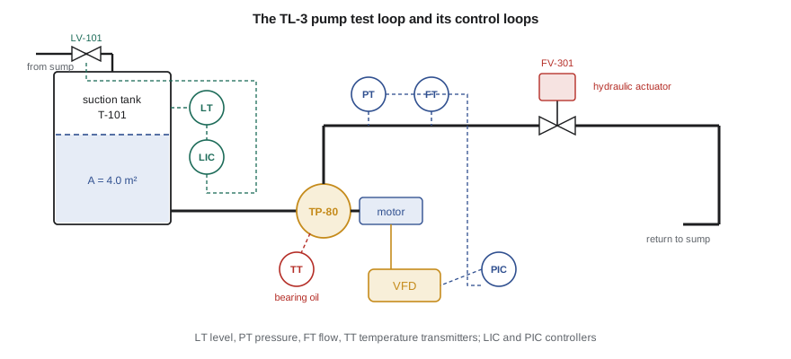
A pump test has to hold its conditions steady while readings are taken. The test procedure, which follows the acceptance-test standard Tidewater's customers specify, requires the flow, the head and the speed to be held within narrow bands for each test point, and it requires the suction conditions to stay constant. On the old stand an operator did this by hand, turning a throttling valve and watching gauges, and a full performance test of one pump took most of a morning. Farah's specification for TL-3 calls for automatic control of four quantities: the level in the suction tank, the pump discharge pressure, the position of a hydraulically actuated throttling valve, and the bearing oil temperature of the pump under test. Each is a dynamic system, and each will be controlled by feedback.
What makes a system dynamic
A system is static when its output depends only on its present input: a pressure gauge with no damping, a lever, a resistor. It is dynamic when its output also depends on its past, because the system stores something. The suction tank stores water, so its level depends on the whole history of inflow and outflow, not just on today's flows. The bearing housing stores heat, so its temperature lags behind changes in friction. The rotor of the pump stores kinetic energy, so its speed cannot change instantly when the motor torque changes. Storage is the common thread: wherever energy or material accumulates, the system has memory, and its behavior is described by differential equations rather than algebraic ones.
The number of independent storage elements sets the order of the system. One tank or one thermal mass gives a first-order system, described by a first-order differential equation and characterized by a single time constant. A mass on a spring, which stores both kinetic and potential energy, gives a second-order system that can oscillate. The test loop as a whole has many stores, but a good model keeps only those that matter at the time scale of interest. The rotor of the TP-80 reaches a new speed in about ten milliseconds once the drive changes its torque; the suction tank takes several minutes to settle after a flow change. A model of the level loop can treat the pump speed as instantaneous, and a model of the speed loop can treat the tank level as constant. Choosing time scales in this way is one of the most useful habits in system dynamics.
Models are built for a purpose
Lucie's first instruction is that every model must answer a question. The same physical tank can be described by a model with one equation or one with a thousand, and the right choice depends on what Owen needs to know. To choose a level controller he needs the relationship between valve opening and tank level over a few minutes. To check whether the tank wall will crack in an earthquake, a structural engineer needs a completely different model of the same tank. A model that tries to answer every question is slow to build, hard to check and usually wrong in ways nobody notices.
The process has six steps, which this course will repeat for every system Owen meets. First, state the purpose: what input, what output, over what time scale and with what accuracy. Second, idealize: replace the real hardware with lumped elements, such as masses, springs, tanks, resistances and thermal capacitances, and write down every assumption. Third, write the equations: conservation laws (mass, energy, momentum) for each store, plus element laws such as Hooke's law or the valve flow equation that relate the variables. Fourth, solve, either analytically or numerically. Fifth, validate: compare the model's predictions with test data, and revisit the assumptions if they disagree. Sixth, use the model, here to design and tune controllers.
| Step | Question to answer | Suction tank example |
|---|---|---|
| Purpose | What do we need to predict, and over what time? | Level response to inflow changes over 1 hour |
| Idealize | Which stores matter? What do we neglect? | One tank; water incompressible; level uniform; no waves |
| Equations | Which balance and which element laws? | Mass balance; drain valve flow q = K√h |
| Solve | Analytic or numeric? | Linearize for analysis; integrate numerically to check |
| Validate | Does the model match a test? | Step the inflow and log the level |
| Use | What decision does the model support? | Controller type and tuning for LIC-101 |
A first model: the suction tank
The suction tank T-101 is a vertical cylinder with a cross-sectional area of 4.0 m², normally holding water about 1.5 m deep. For the first test of the model, the outlet to the test pump is closed and the tank drains by gravity through a manual drain valve to the sump, while the fill valve from the transfer pump supplies an inflow \(q_{in}\). Conservation of mass for an incompressible liquid says that the volume stored changes at the rate inflow minus outflow:
The outflow through the drain valve depends on the level. For turbulent flow through a valve or orifice, the flow is proportional to the square root of the pressure difference across it, and that pressure difference is the hydrostatic head \(\rho g h\). Lumping the constants into a single valve coefficient K gives
This is a nonlinear first-order differential equation. With the drain valve set so that 90 m³/h (0.025 m³/s) leaves the tank at a level of 1.50 m, the coefficient is \(K = 0.025/\sqrt{1.5} = 0.0204\) m^2.5/s. At steady state the level is constant, so inflow equals outflow and \(h = (q_{in}/K)^2\). The square makes the system's sensitivity depend on where it is operating: the same extra inflow raises the level more when the tank is already full than when it is nearly empty.
Linearization
Nonlinear equations are awkward for controller design, because almost all of the design tools in this course, from transfer functions to Bode plots, assume linear systems. The standard remedy is linearization: describe small deviations from a steady operating point with a straight-line approximation of each nonlinear function. Writing \(h = h_0 + \Delta h\) and expanding the square root in a Taylor series about \(h_0\), keeping only the first-order term,
where \(R = 2\sqrt{h_0}/K = 2h_0/q_0\) is the linearized hydraulic resistance of the valve, the change in level per unit change in flow. Here \(R = 2 \times 1.5/0.025 = 120\) s/m². Subtracting the steady-state balance from the full equation leaves a linear equation in the deviation variables:
The product \(\tau = AR = 480\) s, or 8 minutes, is the time constant of the tank. It has a physical meaning that Owen will use again and again: it is the time the tank would take to fill the change in volume if the initial rate of rise continued unchanged. After one time constant a first-order system has completed 63 percent of its response to a step; after four it is within 2 percent of its final value.
# Suction tank T-101 on the TL-3 test loop: a nonlinear model, its linearization and a check against test data
import math
A = 4.0                     # tank cross-section, m^2
h0, q0 = 1.50, 0.025        # normal level (m) and flow through the drain valve (m^3/s, 90 m^3/h)
K = q0 / math.sqrt(h0)      # drain valve coefficient in q = K*sqrt(h), m^2.5/s
R = 2 * h0 / q0             # linearized resistance dh/dq at the operating point, s/m^2
tau = A * R                 # time constant of the linear model, s
print(f"Valve coefficient K = {K:.5f} m^2.5/s")
print(f"Linear resistance R = {R:.0f} s/m^2, time constant tau = A R = {tau:.0f} s ({tau/60:.1f} min)")

def rk4(f, x, t, dt):
    k1 = f(t, x); k2 = f(t + dt/2, x + dt/2*k1); k3 = f(t + dt/2, x + dt/2*k2); k4 = f(t + dt, x + dt*k3)
    return x + dt/6*(k1 + 2*k2 + 2*k3 + k4)

qin = 0.030                 # inflow steps from 0.025 to 0.030 m^3/s at t = 0
nonlin = lambda t, h: (qin - K*math.sqrt(max(h, 0.0))) / A
lin = lambda t, dh: ((qin - q0) - dh / R) / A
h, dh, dt = h0, 0.0, 5.0
rows = []
for n in range(0, 721):
    t = n * dt
    if n % 72 == 0: rows.append((t, h, h0 + dh))
    h = rk4(nonlin, h, t, dt); dh = rk4(lin, dh, t, dt)
print("\n  t (min)   nonlinear h (m)   linear h (m)")
for t, a, b in rows: print(f"  {t/60:6.0f}     {a:8.3f}          {b:8.3f}")
print(f"\nFinal levels: nonlinear {(qin/K)**2:.3f} m, linear {h0 + R*(qin - q0):.3f} m")

# Compare with levels logged on the test floor after the same step (every 6 min)
measured = [1.497, 1.801, 1.948, 2.027, 2.067, 2.081, 2.091, 2.107, 2.103, 2.104, 2.114]
err = [m - r[1] for m, r in zip(measured, rows)]
rms = math.sqrt(sum(e*e for e in err) / len(err))
print(f"RMS difference between the nonlinear model and the logged levels: {rms*1000:.0f} mm")
# A 1.2 % larger valve coefficient explains the lower final level
K2 = K * 1.012
print(f"With K increased by 1.2 %, the predicted final level is {(qin/K2)**2:.3f} m")Valve coefficient K = 0.02041 m^2.5/s
Linear resistance R = 120 s/m^2, time constant tau = A R = 480 s (8.0 min)
t (min) nonlinear h (m) linear h (m)
0 1.500 1.500
6 1.820 1.817
12 1.982 1.966
18 2.066 2.037
24 2.110 2.070
30 2.133 2.086
36 2.146 2.093
42 2.152 2.097
48 2.156 2.099
54 2.158 2.099
60 2.159 2.100
Final levels: nonlinear 2.160 m, linear 2.100 m
RMS difference between the nonlinear model and the logged levels: 43 mm
With K increased by 1.2 %, the predicted final level is 2.109 mThe program integrates both models with the fourth-order Runge-Kutta method, a standard numerical scheme that this course uses throughout because it is accurate and easy to write. For a 20 percent step in inflow, the nonlinear model settles at 2.160 m and the linear model at 2.100 m. The linear model underestimates the rise because the valve's resistance grows as the level rises: at 2.16 m the true slope \(dh/dq\) is about 144 s/m², not 120. The error is 60 mm on a 660 mm change, about 9 percent, which is acceptable for controller design because feedback keeps the level close to the operating point, where the linear model is exact. For large changes in operating point, a controller tuned at one level may need different settings at another, an idea called gain scheduling that returns in Lesson 12.
Validation
Gilles ran the same step on the old tank, which the new one copies, and logged the level every six minutes. The program compares the log with the nonlinear model and finds an RMS difference of 43 mm. The measured level rises a little more slowly and settles lower, near 2.11 m. A model that is consistently off in one direction usually has a wrong parameter rather than a wrong structure. Here, increasing the valve coefficient by only 1.2 percent brings the predicted final level to 2.109 m. Lucie is satisfied: the valve was set by hand, and a 1.2 percent difference in its coefficient is well within the accuracy of that setting. The lesson Owen draws is that validation is not a pass-or-fail exercise but a way of calibrating the model and learning which assumptions matter.
Worked problem
Time constant of a smaller tank
The old stand had a suction tank of 2.5 m² area, run at a level of 1.2 m with 60 m³/h leaving through its drain valve. Find the linearized resistance and the time constant, and estimate how long the level takes to settle after a small change in inflow.
Show solution
- Flow \(q_0 = 60/3600 = 0.01667\) m³/s.
- \(R = 2h_0/q_0 = 2(1.2)/0.01667 = 144\) s/m².
- \(\tau = AR = 2.5 \times 144 = 360\) s, or 6 minutes.
- Settling to within 2 percent takes about \(4\tau = 24\) minutes.
Answer: The smaller tank responds faster, but each unit of flow change moves its level further, since R is larger. Time constant and gain are separate properties, and both matter to the controller.
Linear systems and superposition
Linear models have one property that makes them so valuable: superposition. If input \(u_1\) produces output \(y_1\) and input \(u_2\) produces \(y_2\), then \(au_1 + bu_2\) produces \(ay_1 + by_2\). This means a complicated input can be broken into simple pieces, such as steps, impulses and sine waves, whose responses are known, and the results added. Steps reveal how fast a system is and where it settles; sine waves reveal how it treats each frequency. Lessons 7 and 11 build on these two views. Nonlinear systems obey superposition only approximately, near an operating point, which is exactly what linearization exploits.
Systems are also classified by whether their parameters change with time. The suction tank is time-invariant: a step today produces the same response as a step tomorrow. A tank whose cross-section varied with height, such as a horizontal cylindrical tank, would still be time-invariant but nonlinear in a different way. A rocket burning fuel is time-varying, because its mass changes. Every system in this course is treated as linear and time-invariant (LTI) after linearization, which is the setting in which transfer functions and frequency response are defined.
Numerical simulation
Few nonlinear models can be solved in closed form, and engineers routinely integrate them numerically. The simplest method, Euler's, advances the state by the derivative times the step: \(x_{k+1} = x_k + \Delta t\,f(x_k)\). It is easy to understand but needs very small steps to be accurate. The fourth-order Runge-Kutta method evaluates the derivative four times per step and combines the results, giving errors that shrink with the fourth power of the step size. With a time constant of 480 s, a 5 s step gives results accurate to well under a millimeter. The rule of thumb is to choose a step at most a tenth of the fastest time constant you care about, and to halve it once to confirm the answer does not change.
Simulation also lets Owen include effects that analysis cannot handle easily: valves that saturate fully open or closed, flows that cannot go negative, sensors that read in steps. The programs in this course are short and use only the Python standard library, so each one can be read line by line. In industry the same calculations are usually done with dedicated tools, but understanding what the tool does is the difference between using it and trusting it blindly.
By the end of the first week Owen has a validated model of the tank, a list of the other stores in the loop and a plan for the term. Lessons 2 to 4 model each part of TL-3: the mechanical parts, the fluid and thermal parts, and the electromechanical drive that ties them together. Lessons 5 to 8 develop the mathematics of transfer functions, block diagrams, time response and stability. Lessons 9 to 12 design the controllers.
Common mistakes
MistakeBuilding the most detailed model possible.
InsteadBuild the simplest model that answers the question, and say what it neglects.
MistakeUsing a linear model far from its operating point.
InsteadLinearize about the point where the system will run, and check large changes with the nonlinear model.
MistakeTreating a model as correct because it is based on physics.
InsteadValidate it against a test and calibrate uncertain parameters.
MistakeConfusing a system's time constant with its gain.
Insteadτ says how fast it responds; the gain says how far it moves for a given input.
MistakeChoosing a simulation step without checking it.
InsteadUse a step well below the fastest time constant and confirm that halving it changes nothing.
Summary and key terms
- A dynamic system stores energy or material; its output depends on its history, and it is described by differential equations.
- The order of a model equals the number of independent stores it keeps; time scales decide which to keep.
- Models are built for a purpose: idealize, write balances and element laws, solve, validate and use.
- The suction tank obeys A dh/dt = q_in − K√h; linearized at 1.5 m and 0.025 m³/s it has R = 120 s/m² and τ = AR = 480 s.
- Linearization keeps the first term of a Taylor series about an operating point; it is accurate for small deviations.
- Validation against logged data showed a 1.2 percent error in the valve coefficient, corrected by calibration.
- Dynamic system
- A system whose output depends on past inputs because it stores energy or material.
- Lumped model
- A model that represents distributed properties by a finite number of ideal elements.
- Order
- The number of independent energy or material stores in a model.
- Operating point
- The steady condition about which a nonlinear model is linearized.
- Linearization
- Replacing a nonlinear function by its tangent line or plane at an operating point.
- Deviation variable
- The difference between a variable and its value at the operating point.
- Time constant
- The time for a first-order system to complete 63.2 percent of its step response.
- Hydraulic resistance
- The change in head or pressure per unit change in flow through a restriction.
- Superposition
- The property of linear systems that the response to a sum of inputs is the sum of the responses.
- Validation
- Comparing model predictions with measurements to judge and improve a model.
Practice problems
Work each problem on paper first, then reveal the answer to check.
A tank of 3.0 m² area drains through a valve passing 0.020 m³/s at a level of 2.0 m. Find R and τ.
Show answer
R = 2(2.0)/0.020 = 200 s/m²; τ = 600 s.
For the tank in the last question, how much does the level rise for a small inflow increase of 0.002 m³/s?
Show answer
R Δq = 0.4 m.
What is the order of a model with two tanks and a mass on a spring?
Show answer
Four: one store per tank and two for the mass-spring.
In the program, change the inflow step to 0.027 m³/s. How close are the two models now?
Show answer
Nonlinear 1.750 m, linear 1.740 m: within 10 mm.
Why does the linear tank model underestimate the level rise for a large inflow increase?
Show answer
The true resistance 2h/q grows with level, so the tank rises more than the slope at 1.5 m predicts.
Gilles proposes a 0.5 s simulation step for the tank. Is it necessary?
Show answer
No; with τ = 480 s a 5 s step is already accurate, though a smaller step does no harm.
Lesson quiz · 5 questions
Score 60% or more to complete this lesson.
Create a free account to save your progress, take quizzes and earn a certificate.