
MEC-270 · Lesson 5 of 12 · 22 min
Fluid kinematics
So far the water has been at rest. From here on it moves, and before asking what forces drive the motion we need a language for describing it. That is kinematics: velocity, acceleration, streamlines and the ways a flow can be visualized and classified. Jun Park meets these ideas on his first tour of the raw-water intake, where Hana Lindqvist points out the slow swirl in the intake bay, the smooth acceleration of water into the bellmouth of the suction pipe, and the dye trace that operators once used to check whether chemical feed was mixing properly. Each of those observations is a kinematic description.
Lagrangian and Eulerian descriptions
There are two ways to describe a moving fluid. In the Lagrangian description, we follow individual fluid particles and record each one's position, velocity and acceleration as functions of time, much as we follow a projectile in dynamics. It is natural for tracking a slug of fluoride solution through the plant or a drifting float on the reservoir, but impractical for a whole flow, because a pipe contains an astronomical number of particles.
In the Eulerian description, we fix our attention on points in space and record what happens there as particles pass through: the velocity field \(\mathbf{V}(x, y, z, t)\), the pressure field \(p(x, y, z, t)\), and so on. A flow meter bolted to a pipe and a pressure gauge on a tank wall are Eulerian instruments. Nearly all of fluid mechanics uses the Eulerian view, because engineers care about what happens at the pump inlet or the meter throat, not about the life history of a particular liter of water.
Steady and unsteady flow
A flow is steady if the velocity and other properties at each fixed point do not change with time. Steady does not mean uniform: water speeds up through the venturi throat and slows down after it, but if the pumps run at a constant rate, the speed at the throat is the same at noon as at one o'clock. A flow is unsteady if properties at a point change with time, as they do while a pump starts, a valve closes or a tank drains. Many flows that are unsteady in detail, such as turbulent flow in a pipe, are steady on average and are treated as steady for engineering purposes.
Flows are also classified by how many space coordinates the velocity depends on. Flow in a long straight pipe, far from its entrance, is effectively one-dimensional if we describe it by its average velocity, two-dimensional in the sense that velocity varies with radius, and fully three-dimensional around a bend or a pump impeller. Choosing the simplest description that captures what matters is one of the engineer's most useful skills.
Acceleration of a fluid particle
Newton's second law applies to particles, so to use it in the Eulerian view we need the acceleration of a fluid particle expressed in terms of the velocity field. A particle's velocity changes for two reasons. The field may change with time at a fixed point, which gives the local acceleration. And the particle may move to a place where the velocity is different, even in a steady flow, which gives the convective acceleration. Water entering the venturi throat accelerates even though the flow is steady, because each particle moves into a region of higher speed.
The operator \(D/Dt\) is the material derivative, the rate of change following a particle. The first term is local, the other three are convective. The same operator applies to any property: the rate at which a particle's temperature changes is \(DT/Dt\), which includes both the warming of the water at a fixed point and the particle's movement through a temperature gradient. In one dimension along a pipe, the convective acceleration reduces to \(u\,du/dx\), which is large where the cross-section changes abruptly.
Worked problem
Acceleration toward the intake
Near the intake, a simple model of the flow toward a corner is \(u = kx\), \(v = -ky\), with \(k = 0.5\ \text{s}^{-1}\) and distances in meters. Find the velocity and acceleration of a particle at (2, 1).
Show solution
- Velocity: \(u = 0.5(2) = 1.0\ \text{m/s}\), \(v = -0.5(1) = -0.5\ \text{m/s}\).
- The flow is steady, so the local term is zero. Partial derivatives: \(\partial u/\partial x = k\), \(\partial u/\partial y = 0\), \(\partial v/\partial x = 0\), \(\partial v/\partial y = -k\).
- \(a_x = u\,\partial u/\partial x + v\,\partial u/\partial y = 1.0(0.5) + 0 = 0.50\ \text{m/s}^2\).
- \(a_y = u\,\partial v/\partial x + v\,\partial v/\partial y = 0 + (-0.5)(-0.5) = 0.25\ \text{m/s}^2\).
Answer: The particle accelerates at (0.50, 0.25) m/s² even though the flow is steady. It is speeding up in x as it moves away from the corner and slowing its downward motion as it approaches the wall.
Streamlines, pathlines and streaklines
Three kinds of lines help us visualize a flow. A streamline is a line everywhere tangent to the velocity vector at a given instant. No fluid crosses a streamline, so a bundle of streamlines forms a stream tube that behaves like a pipe with invisible walls. In two dimensions, a streamline satisfies \(dy/dx = v/u\). A pathline is the actual path traced by one particle over time, such as the track of a neutrally buoyant float. A streakline joins all particles that have passed through a given point, which is what you see when dye is injected continuously from a needle or smoke from a chimney.
In steady flow, all three lines coincide: every particle passing a point follows the same path, and that path is tangent to the unchanging velocity field. In unsteady flow they differ, sometimes dramatically. A plume of smoke from a stack on a gusty day forms a wavy streakline, while each smoke particle has traveled a nearly straight pathline. When operators inject dye or salt to check how a tracer moves through a contact tank, they must remember that the pattern they see is a streakline.
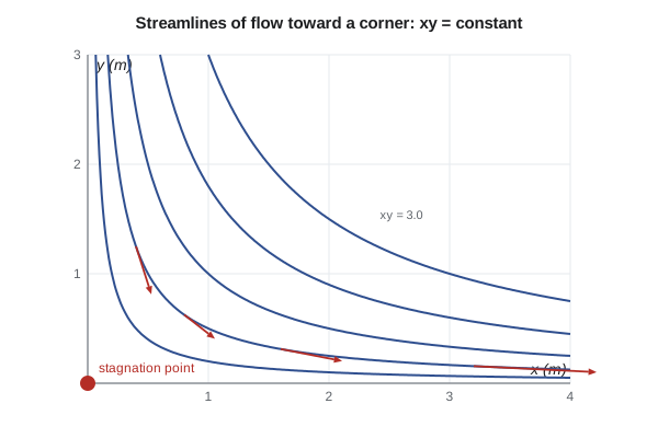
For the corner flow of the example, the streamline equation \(dy/dx = -ky/(kx) = -y/x\) integrates to \(xy = \text{constant}\), a family of hyperbolas. At the origin the velocity is zero. Such a point, where the flow divides and comes to rest, is a stagnation point. Stagnation points appear at the nose of every bluff body, at the center of a jet striking a wall and at the tip of a pitot tube, and the pressure there is the highest in the flow, a fact we use in Lesson 7.
# Velocity, acceleration and streamlines of a 2D flow toward the intake
# Steady stagnation-type flow: u = k*x, v = -k*y  (k in 1/s)
k = 0.5

def vel(x, y):
    return k * x, -k * y

def accel(x, y):
    u, v = vel(x, y)
    du_dx, du_dy = k, 0.0
    dv_dx, dv_dy = 0.0, -k
    ax = u * du_dx + v * du_dy          # convective acceleration (steady flow: no local term)
    ay = u * dv_dx + v * dv_dy
    return ax, ay

for x, y in ((1, 1), (2, 1), (2, 0.5), (4, 0.25)):
    u, v = vel(x, y); ax, ay = accel(x, y)
    print(f"({x},{y}): V = ({u:.2f}, {v:.2f}) m/s, a = ({ax:.3f}, {ay:.3f}) m/s^2")

# Trace a pathline with small time steps (it coincides with a streamline in steady flow)
x, y, t, dt = 0.2, 2.0, 0.0, 0.01
print()
print(" t (s)    x (m)    y (m)    x*y")
for step in range(601):
    if step % 100 == 0:
        print(f"{t:5.1f}  {x:7.3f}  {y:7.3f}  {x*y:6.3f}")
    u, v = vel(x, y)
    # midpoint (RK2) step
    xm, ym = x + 0.5 * dt * u, y + 0.5 * dt * v
    um, vm = vel(xm, ym)
x, y, t = x + dt * um, y + dt * vm, t + dt(1,1): V = (0.50, -0.50) m/s, a = (0.250, 0.250) m/s^2 (2,1): V = (1.00, -0.50) m/s, a = (0.500, 0.250) m/s^2 (2,0.5): V = (1.00, -0.25) m/s, a = (0.500, 0.125) m/s^2 (4,0.25): V = (2.00, -0.12) m/s, a = (1.000, 0.062) m/s^2 t (s) x (m) y (m) x*y 0.0 0.200 2.000 0.400 1.0 0.330 1.213 0.400 2.0 0.544 0.736 0.400 3.0 0.896 0.446 0.400 4.0 1.478 0.271 0.400 5.0 2.436 0.164 0.400 6.0 4.017 0.100 0.400
The program traces a particle released at (0.2, 2.0) by stepping its position forward with the local velocity. The product \(xy\) stays at 0.400 throughout, confirming that the particle follows a streamline, as it must in steady flow. The same stepping method, refined, is how computational fluid dynamics codes trace particles through a simulated flow field.
Flow visualization in practice
Engineers make flows visible in many ways. Dye injection and smoke trace streaklines. Tufts of yarn on a surface show the direction of the flow next to it and reveal regions of separation, where the tufts flutter or point backward. Particle image velocimetry seeds the flow with tiny reflective particles, lights a plane with a laser sheet and photographs it twice in quick succession; software then computes a full velocity field from how far the particles moved. Hydraulic engineers still build physical scale models of intakes and pump sumps to look for vortices that could draw air into a pump, using the similarity rules covered in Fluid Mechanics II.
Computational fluid dynamics now complements those tests. It solves the governing equations on a mesh and displays streamlines, velocity contours and pressure fields. Its pictures are vivid, but they are only as good as the mesh, the turbulence model and the boundary conditions. Hana's rule is that any computed result for a new intake must be checked against a hand calculation of flow rate and average velocity, which needs only the ideas in this lesson and the next.
Rotation, deformation and vorticity
A small element of fluid can translate, rotate and deform as it moves. Its rate of rotation is measured by the vorticity \(\boldsymbol{\omega} = \nabla \times \mathbf{V}\), equal to twice its angular velocity. In two dimensions, the vorticity has a single component, \(\omega_z = \partial v/\partial x - \partial u/\partial y\). A flow with zero vorticity everywhere is irrotational. The corner flow in the example is irrotational, since both cross derivatives are zero; fluid elements there are stretched and squashed but do not spin.
Viscosity creates vorticity at solid walls, where the no-slip condition forces a velocity gradient, and the vorticity spreads outward through the boundary layer. Away from walls, in large reservoirs and in the core of flows through contractions, the flow is often nearly irrotational, and that approximation underlies the Bernoulli equation's use across streamlines. Strong concentrated vorticity, by contrast, forms the swirling vortices that can appear above a pump intake when the submergence is too small, pulling air into the suction pipe and damaging the pump.
| Classification | Meaning | Example at Northside |
|---|---|---|
| Steady | Properties at each point constant in time | Venturi flow at constant pump rate |
| Unsteady | Properties at a point change with time | Backwash tank draining; pump start-up |
| Uniform | Velocity the same at every point along a streamline | Long straight pipe of constant diameter |
| Non-uniform | Velocity changes along a streamline | Venturi contraction; pump inlet bellmouth |
| Irrotational | Zero vorticity | Core flow entering a smooth contraction |
| Rotational | Non-zero vorticity | Boundary layers; intake vortices |
Common mistakes
MistakeAssuming steady flow has no acceleration.
InsteadParticles accelerate convectively wherever velocity changes along their path, even in steady flow.
MistakeTreating a dye streak in unsteady flow as a streamline.
InsteadDye shows a streakline, which coincides with streamlines only in steady flow.
MistakeConfusing uniform and steady flow.
InsteadSteady means no change with time at a point; uniform means no change with position.
MistakeDropping the convective terms in the material derivative.
Insteada = ∂V/∂t + (V·∇)V; both parts matter.
MistakeTrusting a CFD picture without a hand check of flow rate and velocity.
InsteadCheck computed results against simple mass-balance calculations.
Summary and key terms
- The Eulerian description gives velocity and pressure as fields in space and time; the Lagrangian description follows particles.
- Steady flow has no change with time at a fixed point; uniform flow has no change with position.
- Particle acceleration is the material derivative: local plus convective acceleration.
- Streamlines are tangent to velocity; pathlines are particle tracks; streaklines join particles from one point.
- In steady flow, streamlines, pathlines and streaklines coincide.
- Vorticity measures fluid rotation; irrotational flow has zero vorticity.
- Kinematics
- The description of motion without regard to the forces causing it.
- Eulerian description
- Describing a flow by fields of velocity and other properties at fixed points.
- Lagrangian description
- Describing a flow by following individual fluid particles.
- Steady flow
- Flow whose properties at each point do not change with time.
- Material derivative
- The rate of change following a fluid particle, D/Dt = ∂/∂t + V·∇.
- Convective acceleration
- Acceleration of a particle caused by moving to a place where the velocity differs.
- Streamline
- A line everywhere tangent to the velocity vector at an instant.
- Pathline
- The trajectory of a single fluid particle.
- Streakline
- The line joining all particles that have passed through one point.
- Stagnation point
- A point in a flow where the velocity is zero.
- Vorticity
- The curl of the velocity field, equal to twice the local angular velocity of the fluid.
Practice problems
Work each problem on paper first, then reveal the answer to check.
A velocity field is u = 2x, v = −2y (m/s). Find the acceleration at (1, 3).
Show answer
a_x = u ∂u/∂x = 2(2) = 4 m/s²; a_y = v ∂v/∂y = (−6)(−2) = 12 m/s².
Water flows steadily along a contraction where u = 1 + 0.5x m/s. Find the acceleration at x = 2 m.
Show answer
a = u du/dx = 2(0.5) = 1.0 m/s².
Find the streamlines of u = y, v = x.
Show answer
dy/dx = x/y gives y² − x² = constant, a family of hyperbolas.
Is the flow u = −ky, v = kx irrotational?
Show answer
ω_z = k − (−k) = 2k, so it rotates like a rigid body; it is rotational.
Smoke from a stack on a day of steady wind direction forms a straight plume. What does that tell you about the flow?
Show answer
It is nearly steady, so the streakline, pathlines and streamlines coincide.
In the program, release the particle at (0.1, 4.0). What value of xy does it keep?
Show answer
0.400, the same streamline, so it follows the same path from farther up.
Lesson quiz · 5 questions
Score 60% or more to complete this lesson.
Create a free account to save your progress, take quizzes and earn a certificate.