Errors and floating point

Almost every number an engineer computes today comes out of a computer: the stresses from a finite element model, the flows in a pipe network, the trajectory of a rocket, the forecast from a reservoir simulator. None of these numbers is exact. Numerical methods are the techniques that turn mathematical problems into arithmetic a computer can do, and the first skill they demand is understanding error: where it comes from, how big it is, and how to keep it from growing until the answer is meaningless.

This chapter sets up the vocabulary for the whole course: absolute and relative error, the sources of error, how computers store real numbers, round-off and truncation error, catastrophic cancellation and conditioning.

Measuring error

If p is the true value and \(\tilde{p}\) an approximation, the absolute error and relative error are

Relative error is usually more meaningful. An error of 1 mm is negligible in the span of a bridge and disastrous in the bore of an engine cylinder. A relative error of about \(5 \times 10^{-n}\) corresponds to roughly n correct significant figures.

In practice the true value is unknown, so iterative methods estimate the error from successive approximations, stopping when the approximate relative error falls below a tolerance:

Where errors come from

A numerical result passes through several stages, and each adds error:

• Modeling error: the equations simplify reality (a beam treated as perfectly elastic, air resistance ignored, a soil layer assumed uniform).
• Data error: inputs are measured or estimated (loads, material properties, flow rates), each with its own uncertainty.
• Truncation error: the numerical method approximates an exact mathematical operation, such as a derivative by a finite difference, an integral by a sum, or an infinite series by a few terms.
• Round-off error: the computer stores and computes with a finite number of digits.

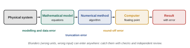
The numerical analyst controls the last two. Neither is useful to reduce far below the first two: computing a stress to 12 significant figures is pointless if the load is known to 10%. But truncation and round-off can also grow far beyond the data error if a method is badly chosen, and that is what this course teaches you to prevent.

How computers store numbers

Computers store real numbers in binary floating point, a kind of scientific notation in base 2:

The IEEE 754 double-precision format, used by Python, MATLAB, Excel and almost all engineering software, has 64 bits: 1 for the sign, 11 for the exponent e (about −1022 to 1023) and 52 for the fraction. This gives about 16 significant decimal digits and a range from about \(10^{-308}\) to \(10^{308}\). Single precision (32 bits, 24 significant bits) gives only about 7 digits and is used where memory or speed matters more, as in graphics cards and many sensors.

The key number is machine epsilon, the gap between 1 and the next larger representable number:

Every arithmetic operation is rounded to the nearest representable number, so each one can introduce a relative error of up to about \(\varepsilon_{\text{mach}}/2\). Representable numbers are not evenly spaced: the gaps grow in proportion to the size of the number, which is what keeps the relative error roughly constant.

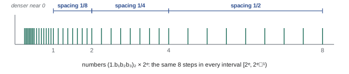
Many simple decimal fractions have no exact binary representation, just as 1/3 has none in decimal. The number 0.1 in binary is 0.000110011001100… repeating forever, so it is stored rounded. This is why, in Python, 0.1 + 0.2 gives 0.30000000000000004 and the test 0.1 + 0.2 == 0.3 is False.

Round-off error accumulates

One rounding error of \(10^{-16}\) is harmless. Trouble comes when millions of them accumulate, or when a calculation magnifies one.

A famous financial example: in 1982 the Vancouver Stock Exchange started a new index at 1000.000 and recomputed it thousands of times a day, truncating (chopping) each result to three decimals instead of rounding. Each chop lost a little, always in the same direction. By late 1983 the index stood at about 524.8, when the correctly computed value was about 1098.9.

Catastrophic cancellation

Subtracting two nearly equal numbers destroys significant figures. If a = 1.23456789 and b = 1.23456700, each known to 9 digits, then a − b = 0.00000089 has only 2 significant digits left. The subtraction itself is exact; it exposes the rounding errors that were already in a and b.

Other common fixes: compute \(1 - \cos x\) for small x as \(2\sin^2(x/2)\) (at \(x = 10^{-8}\) the direct form gives exactly 0, the rewritten one \(5 \times 10^{-17}\)), and use library functions such as log1p(x) and expm1(x), which are designed for arguments near zero.

Truncation error and Taylor series

Truncation error comes from approximating an infinite process by a finite one. Taylor series (MATH-101) are the main tool for analyzing it:

Cutting the series after a few terms leaves an error about the size of the first omitted term. For example, \(e^{0.5}\) from the series \(1 + x + x^2/2! + \cdots\) has errors of 0.149, 0.024, 0.0029 and 0.00028 after 2, 3, 4 and 5 terms: each extra term buys about one more digit.

Finite differences and the best step size

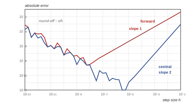
Rearranging the Taylor series gives the forward difference approximation of a derivative and its truncation error:

Subtracting the series for \(f(x - h)\) from that for \(f(x + h)\) cancels the \(h^2\) terms and gives the more accurate central difference:

The notation O(h) means the error shrinks in proportion to h; O(h²) means it shrinks with h²: halving h divides the error by 4. That is the order of the method.

But h cannot be made arbitrarily small. The numerator subtracts two nearly equal values, so its round-off error is about \(\varepsilon_{\text{mach}}|f|\), and dividing by a tiny h magnifies it. Total error is truncation (falling with h) plus round-off (rising as h shrinks), and there is a best h in between.

Conditioning and stability

Two ideas separate the problem from the method. A problem is ill-conditioned if small changes in the input cause large changes in the exact answer. For a function, the condition number compares relative changes:

With κ = 1000, a relative input error of \(10^{-6}\) can become \(10^{-3}\) in the output, whatever method is used. Examples are tan x near π/2, the roots of polynomials with clustered roots, and the linear systems of Lesson 3 whose matrices are nearly singular.

A method (algorithm) is stable if it does not magnify the round-off errors it creates, and unstable if it does. The naive quadratic formula above is an unstable algorithm for a well-conditioned problem: the roots themselves are not sensitive to the coefficients, but the subtraction in the formula is. Good numerical practice means using stable algorithms and recognising ill-conditioned problems, where the remedy is better data or a reformulated problem rather than more digits.

import math
import numpy as np

print(0.1 + 0.2, 0.1 + 0.2 == 0.3, math.isclose(0.1 + 0.2, 0.3))
print("double eps:", np.finfo(float).eps, " single eps:", np.finfo(np.float32).eps)

# small root of x^2 + 1e8 x + 1 = 0
a, b, c = 1.0, 1e8, 1.0
d = math.sqrt(b*b - 4*a*c)
print("naive :", (-b + d) / (2*a))
print("stable:", (2*c) / (-b - d))

# best step for a central difference
for h in [1e-2, 1e-5, 1e-8, 1e-11]:
    est = (math.sin(1 + h) - math.sin(1 - h)) / (2*h)
    print(f"h = {h:.0e}  error = {abs(est - math.cos(1)):.1e}")

Output: 0.30000000000000004 False True; double eps: 2.220446049250313e-16, single eps: 1.1920929e-07; naive: -7.450580596923828e-09, stable: -1e-08; central difference errors 9.0e-06, 1.1e-11, 2.6e-09 and 1.2e-06 for h = 10⁻², 10⁻⁵, 10⁻⁸ and 10⁻¹¹: best near h = 10⁻⁵, then growing again.