Numerical optimization

Design is optimization: choosing the pipe diameter with the lowest lifetime cost, the truss member sizes with the least weight, the controller gains with the best response, the model parameters that best fit the data, the production plan with the most profit. Calculus (MATH-209) characterizes optima by a zero gradient and gives exact answers for small, smooth problems. Real problems have many variables, functions that can only be evaluated by running a simulation, constraints of every kind and sometimes many local optima. This lesson develops the numerical methods used in practice: golden-section search in one variable; gradient-based methods (steepest descent, Newton, quasi-Newton) and the derivative-free Nelder-Mead method in several; nonlinear least squares for fitting models; linear programming and penalty methods for constrained problems; and strategies for problems with many local minima. It builds on root finding (Lesson 2), since a minimum is a root of the gradient, and on linear systems (Lesson 3), which every Newton step solves.

One variable: golden-section search

If a function has a single minimum in an interval \([a, b]\) (it is unimodal there), the minimum can be trapped by evaluating the function at two interior points and discarding the part of the interval that cannot contain it, much as bisection traps a root. Golden-section search places the interior points at fractions 0.382 and 0.618 of the interval. After each comparison the interval shrinks to 0.618 of its length, and one of the old interior points lands exactly where a new one is needed, so each step costs just one new function evaluation. The golden ratio \((\sqrt{5} - 1)/2 = 0.618\) is the unique ratio with this reuse property.

Golden-section search needs no derivatives and cannot fail on a unimodal function, but it converges only linearly. Library routines (Brent's method, scipy.optimize.minimize_scalar) combine it with parabolic interpolation, fitting a parabola through three points and jumping to its vertex, which converges much faster near a smooth minimum, while keeping golden-section steps as a safeguard.

import math

# Annual cost of the pipeline per m of length: capital (grows with D) + pumping energy (falls as 1/D^5)
def cost(D):
    return 400 * D + 0.02 / D**5

def golden(f, a, b, tol=1e-5):
    g = (math.sqrt(5) - 1) / 2          # 0.618...
    c, d = b - g * (b - a), a + g * (b - a)
    fc, fd = f(c), f(d)
    evals = 2
    while b - a > tol:
        if fc < fd:
            b, d, fd = d, c, fc
            c = b - g * (b - a)
            fc = f(c)
        else:
            a, c, fc = c, d, fd
            d = a + g * (b - a)
            fd = f(d)
        evals += 1
    return (a + b) / 2, evals

D, n = golden(cost, 0.05, 1.0)
print(f"Golden section: D = {D:.4f} m after {n} evaluations, cost = {cost(D):.1f} dollars per m per year")
print(f"Exact (from dC/dD = 0): D = {(0.1 / 400)**(1 / 6):.4f} m")
for Dt in [0.20, 0.25, 0.30]:
    print(f"  D = {Dt:.2f} m: cost = {cost(Dt):.1f}")

Golden section: D = 0.2510 m after 26 evaluations, cost = 120.5 dollars per m per year
Exact (from dC/dD = 0): D = 0.2510 m
  D = 0.20 m: cost = 142.5
  D = 0.25 m: cost = 120.5
  D = 0.30 m: cost = 128.2

Several variables: gradient-based methods

MATH-209 introduced steepest descent, which steps in the direction \(-\nabla f\), and Newton's method, which steps to the minimum of the local quadratic model by solving \(H\mathbf{p} = -\nabla f\) with the Hessian matrix H. Practical versions add two ingredients:

• A line search: rather than a fixed step, choose the step length along the search direction to reduce f sufficiently (the Wolfe conditions formalize "sufficiently"). This makes methods robust far from the optimum.
• A good search direction without the full Hessian. Quasi-Newton methods, of which BFGS is the most widely used, build up an approximation to H (or its inverse) from the changes in the gradient between steps. They need only gradients, cost \(O(n^2)\) per step, and converge superlinearly. For very large problems, limited-memory BFGS (L-BFGS) stores only a few recent vectors, and the nonlinear conjugate gradient method needs only a handful of vectors in total.

Gradients can be supplied by hand, computed by finite differences (Lesson 1; n + 1 function evaluations per gradient, with round-off limiting accuracy), or computed exactly and cheaply by automatic differentiation, which applies the chain rule to the computer program itself. Automatic differentiation is what makes it practical to train neural networks with millions of parameters.

Derivative-free methods

When f comes from a simulation or an experiment, gradients may be unavailable or noisy. The Nelder-Mead method keeps a simplex of n + 1 points (a triangle in two dimensions) and repeatedly reflects the worst point through the centroid of the others, expanding, contracting or shrinking the simplex as the function values dictate, so that it tumbles downhill and finally shrinks around the minimum. It is robust and easy to use, but slow in high dimensions and without convergence guarantees.

import numpy as np
from scipy.optimize import minimize, rosen, rosen_der, rosen_hess

x0 = np.array([-1.2, 1.0])            # classic hard start for the Rosenbrock valley
for method in ["Nelder-Mead", "CG", "BFGS", "trust-exact"]:
    kw = {}
    if method in ("CG", "BFGS", "trust-exact"):
        kw["jac"] = rosen_der
    if method == "trust-exact":
        kw["hess"] = rosen_hess
    r = minimize(rosen, x0, method=method, **kw)
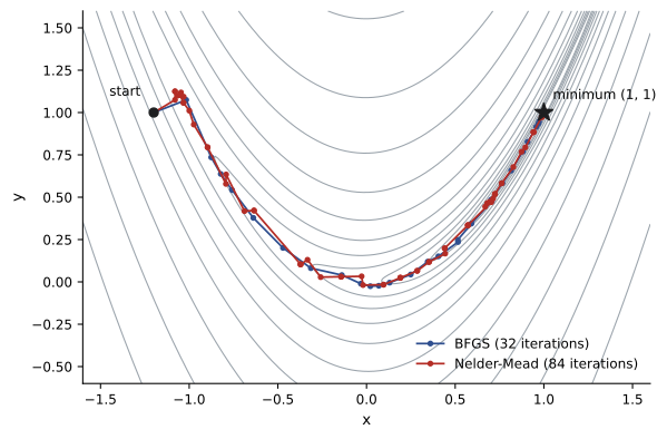
    print(f"{method:12s} x = ({r.x[0]:.6f}, {r.x[1]:.6f})  f evals {r.nfev:4d}  iterations {r.nit:4d}")

Nelder-Mead  x = (1.000022, 1.000042)  f evals  159  iterations   85
CG           x = (1.000000, 1.000000)  f evals   78  iterations   36
BFGS         x = (1.000000, 1.000000)  f evals   39  iterations   32
trust-exact  x = (1.000000, 1.000000)  f evals   26  iterations   25

The Rosenbrock function is a standard test because its curved, narrow valley defeats naive methods. All four methods succeed, but the work differs: Nelder-Mead needs the most function evaluations and stops slightly short of the exact minimum, while the methods that use gradient and Hessian information converge precisely with far fewer. In engineering design, where one function evaluation may be an hour-long simulation, that difference decides what is feasible.

Nonlinear least squares

Fitting a model \(y = g(x; \boldsymbol{\beta})\) with parameters \(\boldsymbol{\beta}\) to data minimizes the sum of squared residuals \(S = \sum r_i^2\), with \(r_i = y_i - g(x_i; \boldsymbol{\beta})\). When g is linear in the parameters, this is a linear least-squares problem (Lesson 5). When it is not, as for exponential decay, a reaction rate with an activation energy or a saturation curve, the Gauss-Newton method linearizes the residuals about the current estimate using their Jacobian matrix J, \(J_{ij} = \partial r_i/\partial\beta_j\), and solves a linear least-squares problem for the step:

The Levenberg-Marquardt method adds a damping term, \((J^TJ + \mu I)\Delta\boldsymbol{\beta} = -J^T\mathbf{r}\), which turns the step toward steepest descent when far from the solution and toward Gauss-Newton when close. It is the algorithm behind scipy.optimize.curve_fit and most curve-fitting software. Good starting values matter: estimate them from the physics or from a rough plot.

Constrained optimization

Linear programming

When the objective and all constraints are linear, the problem is a linear program. The feasible region is a polygon (a polytope in higher dimensions), and the optimum always lies at a corner. The simplex method moves from corner to corner, improving the objective at each step; interior-point methods cut through the middle. Both solve problems with millions of variables, and linear programming is used to schedule production, plan electricity generation, route deliveries and blend materials. Its dual variables, or shadow prices, are the Lagrange multipliers of MATH-209: the value of one more unit of each constrained resource.

from scipy.optimize import linprog

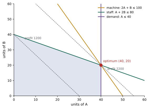
# A plant makes two products. Profit: 40 per unit of A, 30 per unit of B.
# Machine hours: 2A + 1B <= 100; staff hours: 1A + 2B <= 80; demand for A <= 40.
# linprog minimizes, so negate the profit.
res = linprog(c=[-40, -30], A_ub=[[2, 1], [1, 2], [1, 0]], b_ub=[100, 80, 40], bounds=[(0, None), (0, None)])
A, B = res.x
print(f"Make {A:.1f} of A and {B:.1f} of B for a profit of {-res.fun:.0f}")
print("Shadow prices (profit per extra hour or unit):", [round(float(-v), 2) for v in res.ineqlin.marginals])

Make 40.0 of A and 20.0 of B for a profit of 2200
Shadow prices (profit per extra hour or unit): [0.0, 15.0, 25.0]

The optimum is at the corner where staff hours and the demand limit for A are both binding. An extra staff hour would be worth $15 and an extra unit of demand for A $25, while extra machine time is worth nothing at this corner, because the other two constraints already pin the answer. Shadow prices like these tell a manager where investment pays.

Nonlinear constraints

For general constrained problems, two families of methods dominate. Penalty methods add a term to the objective that grows when constraints are violated, \(f + \tfrac{\mu}{2}\sum g_i^2\), and solve a sequence of unconstrained problems with increasing μ; they are simple but become ill-conditioned (Lesson 3) as μ grows. Sequential quadratic programming (SQP) solves, at each step, a quadratic approximation of the problem with linearized constraints, and is the standard method for smooth engineering design problems (scipy.optimize.minimize with method SLSQP or trust-constr).

Local and global minima

Every method above finds a local minimum, the bottom of whichever valley it starts in. Many engineering problems, such as structural layout, the placement of sensors or the tuning of complex models, have many local minima. Common strategies are multistart (run a local method from many random starting points and keep the best), and stochastic global methods such as simulated annealing, genetic algorithms and particle swarm optimization, which accept occasional uphill moves to escape local valleys. None can guarantee the global optimum in general, and all need many function evaluations, so it pays to use physical insight to start near a good design and to check whether the answer makes engineering sense.