Shortest paths and graph algorithms

When you ask a map application for directions, a router forwards a packet across the internet, or a game character walks around an obstacle, a shortest-path computation is running underneath. The problem is easy to state: in a graph whose edges have lengths, find the route of least total length between two vertices. This lesson treats the unweighted case, solved by breadth-first search, and the weighted case with nonnegative lengths, solved by Dijkstra's algorithm, and proves both correct. It then looks at negative lengths, at all-pairs distances, and at the trick that lets such algorithms run on graphs with millions of vertices. The careful analysis of running times and data structures belongs to CMPUT-204; the focus here is on why the algorithms give the right answer.

Distance in a graph

In an unweighted graph, the distance \(d(u, v)\) is the number of edges on a shortest path from \(u\) to \(v\), and \(\infty\) if there is no path. In a weighted graph, each edge \(e\) has a length \(w(e)\), the length of a path is the sum of the lengths of its edges, and \(d(u, v)\) is the least length of a path from \(u\) to \(v\). When all lengths are positive, distance behaves like distance in geometry: \(d(u, v) \ge 0\) with equality only when \(u = v\), \(d(u, v) = d(v, u)\) in an undirected graph, and the triangle inequality \(d(u, w) \le d(u, v) + d(v, w)\) holds, because a shortest route from \(u\) to \(v\) followed by one from \(v\) to \(w\) is one possible route from \(u\) to \(w\).

The key structural fact is that shortest paths are made of shortest paths. If \(P\) is a shortest path from \(s\) to \(t\) and \(v\) is a vertex on it, then the part of \(P\) from \(s\) to \(v\) is a shortest path from \(s\) to \(v\). Otherwise we could replace that part by a shorter one and get a shorter route to \(t\). This optimal substructure is what makes efficient algorithms possible: the distance to a vertex can be built from the distances to its neighbors, \(d(s, v) = \min_{u} \big(d(s, u) + w(uv)\big)\), the minimum over all neighbors \(u\) of \(v\).

Breadth-first search finds unweighted distances

Breadth-first search from \(s\), met in Lesson 8, visits vertices in layers. Layer 0 is \(\{s\}\), and layer \(k + 1\) is the set of unvisited vertices adjacent to some vertex in layer \(k\). Recording for each vertex the vertex it was discovered from gives a breadth-first search tree.

Theorem. In an unweighted graph, breadth-first search from \(s\) places each vertex \(v\) reachable from \(s\) in layer \(d(s, v)\), and the path to \(v\) in the search tree is a shortest path.

Proof by induction on \(k\): we show that layer \(k\) is exactly the set of vertices at distance \(k\). This is true for \(k = 0\). Suppose it is true for all layers up to \(k\). A vertex \(v\) in layer \(k + 1\) has a neighbor in layer \(k\), at distance \(k\), so \(d(s, v) \le k + 1\); and \(v\) was not in an earlier layer, so by the hypothesis \(d(s, v) > k\). Hence \(d(s, v) = k + 1\). Conversely, if \(d(s, v) = k + 1\), the vertex before \(v\) on a shortest path is at distance \(k\), so it is in layer \(k\), and \(v\), which is not in an earlier layer, is discovered from it and placed in layer \(k + 1\).

Breadth-first search uses a queue: vertices are processed first in, first out, which is what produces the layers. It runs in time proportional to \(n + m\), so it handles large graphs easily. Social networks use it to compute degrees of separation. The six degrees of separation idea comes from Stanley Milgram's letter-forwarding experiments of 1967, and a 2011 study of 721 million Facebook users found an average distance of about 4.7.

Dijkstra's algorithm

With lengths on the edges, the fewest edges is no longer the shortest route; a direct road over a mountain may be longer than two roads around it. Edsger Dijkstra published his algorithm in 1959, and later said he had designed it in about twenty minutes while sitting at a café in Amsterdam, without pencil and paper. It assumes every edge length is nonnegative.

The algorithm keeps a tentative distance \(D(v)\) for every vertex, starting with \(D(s) = 0\) and \(D(v) = \infty\) for the others, and a set \(F\) of finished vertices, initially empty. It repeats one step until every vertex is finished:

• Choose the unfinished vertex \(u\) with the smallest tentative distance \(D(u)\), and mark it finished.

• For each edge \(uv\) to an unfinished vertex \(v\), if \(D(u) + w(uv) < D(v)\), set \(D(v) = D(u) + w(uv)\) and record \(u\) as the predecessor of \(v\). This update is called relaxing the edge.

At the end \(D(v) = d(s, v)\) for every vertex, and following predecessors back from \(v\) traces a shortest path. The predecessor edges form a shortest-path tree rooted at \(s\), which is in general different from the minimum spanning tree of Lesson 9.

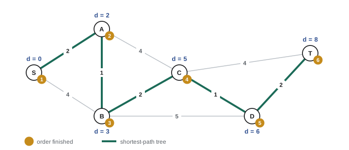
Theorem. If all edge lengths are nonnegative, then when Dijkstra's algorithm finishes a vertex \(u\), its tentative distance \(D(u)\) equals the true distance \(d(s, u)\).

Proof. Throughout the algorithm, every finite \(D(v)\) is the length of an actual path from \(s\) to \(v\), so \(D(v) \ge d(s, v)\) always. Suppose, for a contradiction, that some vertex is finished with \(D(u) > d(s, u)\), and let \(u\) be the first such vertex. Take a shortest path \(P\) from \(s\) to \(u\). It starts in the finished set, since \(s\) is finished first with \(D(s) = 0\), and ends outside it at the moment \(u\) is chosen. Let \(y\) be the first vertex on \(P\) that is not finished, and \(x\) the vertex just before it, which is finished. When \(x\) was finished, its distance was correct because \(u\) is the first exception, and the edge \(xy\) was relaxed, so \(D(y) \le d(s, x) + w(xy) = d(s, y)\), using the fact that the part of \(P\) up to \(y\) is a shortest path. Since lengths are nonnegative, \(d(s, y) \le d(s, u)\), because \(y\) comes before \(u\) on \(P\). Putting these together, \(D(y) \le d(s, y) \le d(s, u) < D(u)\). But the algorithm chose \(u\) as the unfinished vertex of smallest tentative distance, so \(D(u) \le D(y)\). This contradiction proves the theorem.

The proof uses nonnegativity at exactly one point: the claim that a vertex further along a shortest path is at least as far away. With a negative edge this fails, and so can the algorithm. In the graph with edges \(s \to a\) of length 2, \(s \to b\) of length 3 and \(b \to a\) of length \(-2\), Dijkstra finishes \(a\) with distance 2 before discovering the path through \(b\) of length 1.

Negative lengths and all pairs

Negative lengths are not just a curiosity. If edges represent currency exchanges with length equal to minus the logarithm of the exchange rate, a path's length is minus the logarithm of the product of rates, so a negative cycle is a sequence of trades that ends with more money than it started with. With negative edges but no negative cycles, the Bellman–Ford algorithm, from the work of Richard Bellman (1958) and Lester Ford (1956), finds shortest paths by relaxing every edge \(n - 1\) times. That is enough because a shortest path uses at most \(n - 1\) edges, and after round \(k\) every distance achievable with at most \(k\) edges has been found. One more round detects a negative cycle: if any distance still improves, one exists. When a negative cycle is reachable, shortest paths are not defined, since going around the cycle again always gives a shorter walk.

Sometimes we want the distance between every pair of vertices, as in the mileage table on a road map. The Floyd–Warshall algorithm (1962) computes all of them with a three-line triple loop: for each vertex \(k\) in turn, it allows \(k\) as an intermediate stop and updates \(d(i, j) = \min\big(d(i, j), d(i, k) + d(k, j)\big)\). After considering all \(k\), every pair has its shortest distance. The correctness proof is an induction on the set of allowed intermediate vertices, a typical example of dynamic programming.

import heapq
from collections import deque

def bfs_dist(adj, s):
    dist = {s: 0}; queue = deque([s])
    while queue:
        u = queue.popleft()
        for v in adj[u]:
            if v not in dist:
                dist[v] = dist[u] + 1; queue.append(v)
    return dist

def dijkstra(adj, s):
    dist, prev = {s: 0}, {s: None}
    heap, done = [(0, s)], set()
    order = []
    while heap:
        d, u = heapq.heappop(heap)
        if u in done:
            continue
        done.add(u); order.append(u)
        for v, w in adj[u]:
            if v not in done and d + w < dist.get(v, float("inf")):
                dist[v] = d + w; prev[v] = u
                heapq.heappush(heap, (d + w, v))
    return dist, prev, order

def path_to(prev, t):
    p = []
    while t is not None:
        p.append(t); t = prev[t]
    return p[::-1]

def bellman_ford(vertices, edges, s):
    dist = {v: float("inf") for v in vertices}; dist[s] = 0
    for _ in range(len(vertices) - 1):
        for u, v, w in edges:
            if dist[u] + w < dist[v]:
                dist[v] = dist[u] + w
    negative_cycle = any(dist[u] + w < dist[v] for u, v, w in edges)
    return dist, negative_cycle

def floyd_warshall(vertices, edges):
    d = {(i, j): 0 if i == j else float("inf") for i in vertices for j in vertices}
    for u, v, w in edges:
        d[u, v] = min(d[u, v], w)
    for k in vertices:
        for i in vertices:
            for j in vertices:
                if d[i, k] + d[k, j] < d[i, j]:
                    d[i, j] = d[i, k] + d[k, j]
    return d

grid = {(r, c): [(r + dr, c + dc) for dr, dc in ((1, 0), (-1, 0), (0, 1), (0, -1))
                 if 0 <= r + dr < 4 and 0 <= c + dc < 4] for r in range(4) for c in range(4)}
print("BFS distance across a 4x4 grid:", bfs_dist(grid, (0, 0))[(3, 3)])

E = [("S","A",2),("S","B",4),("A","B",1),("A","C",4),("B","C",2),
     ("B","D",5),("C","D",1),("C","T",4),("D","T",2)]
adj = {}
for u, v, w in E:
    adj.setdefault(u, []).append((v, w)); adj.setdefault(v, []).append((u, w))
dist, prev, order = dijkstra(adj, "S")
print("Dijkstra order:", order)
print("distances:", dict(sorted(dist.items())))
print("route to T:", path_to(prev, "T"))

neg = [("s","a",2), ("s","b",3), ("b","a",-2)]
print("Bellman-Ford with a negative edge:", bellman_ford("sab", neg, "s"))
cyc = [("x","y",1), ("y","z",-3), ("z","x",1)]
print("negative cycle detected:", bellman_ford("xyz", cyc, "x")[1])

V = "SABCDT"
both = E + [(v, u, w) for u, v, w in E]
d = floyd_warshall(V, both)
print("all-pairs row for D:", [d["D", j] for j in V])

BFS distance across a 4x4 grid: 6
Dijkstra order: ['S', 'A', 'B', 'C', 'D', 'T']
distances: {'A': 2, 'B': 3, 'C': 5, 'D': 6, 'S': 0, 'T': 8}
route to T: ['S', 'A', 'B', 'C', 'D', 'T']
Bellman-Ford with a negative edge: ({'s': 0, 'a': 1, 'b': 3}, False)
negative cycle detected: True
all-pairs row for D: [6, 4, 3, 1, 0, 2]

Making it fast on real maps

Dijkstra's algorithm explores outward from the start in every direction, like a ripple in a pond, finishing vertices in order of distance. On a continental road network with tens of millions of intersections that is too slow for an interactive query. The A* search algorithm, introduced by Peter Hart, Nils Nilsson and Bertram Raphael in 1968, steers the search toward the target by adding to each tentative distance an estimate of the remaining distance, such as the straight-line distance to the destination. If the estimate never overestimates, A* still returns a shortest path, and it explores far fewer vertices. Modern route planners go further and preprocess the map, for example by ranking intersections by importance so that long queries can climb onto the highways quickly; queries that would take seconds with plain Dijkstra then take milliseconds.

Internet routing uses shortest paths directly. In link-state protocols such as OSPF, every router learns the whole network map and runs Dijkstra's algorithm on it. In distance-vector protocols, each router repeatedly tells its neighbors its current distance estimates, and each one updates using \(d(s, v) = \min_u \big(w(su) + d(u, v)\big)\), which is Bellman–Ford carried out by many machines at once.