
MATH-209 · Lesson 12 of 12 · 29 min
Case studies and course project
This course has built the calculus of several variables step by step: functions and their graphs, curves and motion, partial derivatives and optimization, multiple integrals and changes of variables, line and surface integrals, the theorems of Green, Gauss and Stokes, and their use in fluid mechanics and electromagnetism. Real engineering questions rarely announce which of these tools they need. This lesson works through three case studies that each combine several lessons: the wind force and overturning moment on a tall building, the best tilt for a solar panel, and laminar flow of oil in a pipe. It then summarizes the common approach, sets out the course project and looks ahead to the courses that rely on this one.
Case study 1: wind load on a tall building
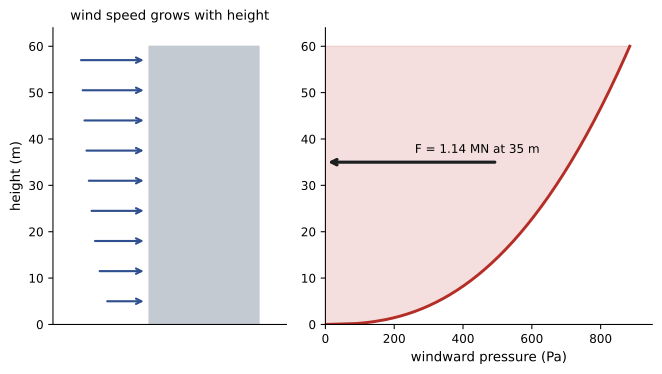
Wind speed increases with height above the ground because the ground slows the air near it. A common model is the power law \(v(z) = v_{10}(z/10)^{\alpha}\), where \(v_{10}\) is the speed at 10 m and the exponent α depends on the terrain (about 0.15 over open water, 0.2 to 0.3 over suburbs and cities). The pressure on the windward face is \(p = C_p\,\tfrac{1}{2}\rho v^2\), with a pressure coefficient \(C_p\) of about 0.8. The total force and the overturning moment about the base are integrals over the face (Lesson 5), and the height of the resultant follows from the ratio, exactly as for the center of pressure on a gate (Lesson 6).
Worked problem
Force and moment on a tower
A building face is 30 m wide and 60 m tall. The wind is 30 m/s at 10 m height with α = 0.2, ρ = 1.2 kg/m³ and C_p = 0.8. Find the total force on the face, the overturning moment about the base and the height of the resultant.
Show solution
- Dynamic pressure: \(q(z) = \tfrac{1}{2}(1.2)(30)^2(z/10)^{0.4} = 540\,(z/10)^{0.4}\) Pa.
- Force: \(F = C_pB\int_0^{60} q\,dz = 0.8 \times 30 \times 540 \times 10^{-0.4} \times \dfrac{60^{1.4}}{1.4} = 1.14\) MN.
- Moment: \(M = C_pB\int_0^{60} q\,z\,dz = 0.8 \times 30 \times 540 \times 10^{-0.4} \times \dfrac{60^{2.4}}{2.4} = 39.8\) MN·m.
- Height of the resultant: \(M/F = 60 \times 1.4/2.4 = 35.0\) m.
Answer: A force of about 1.14 MN acting 35 m above the ground, giving an overturning moment of 39.8 MN·m. The resultant acts above mid-height because the upper floors see faster wind. Building codes, including the National Building Code of Canada, use a similar height-dependent exposure factor, plus gust and shape factors, to set design wind pressures.
import numpy as np

rho, v10, alpha, Cp = 1.2, 30.0, 0.2, 0.8
B, H = 30.0, 60.0
z = np.linspace(0, H, 6001)
q = 0.5 * rho * (v10 * (z / 10)**alpha)**2          # dynamic pressure, Pa

F = Cp * B * np.trapezoid(q, z)
M = Cp * B * np.trapezoid(q * z, z)
k = 0.5 * rho * v10**2 * 10**(-2 * alpha)
F_exact = Cp * B * k * H**(1 + 2 * alpha) / (1 + 2 * alpha)
print(f"Numerical:   F = {F / 1e6:.3f} MN, M = {M / 1e6:.1f} MN m, height {M / F:.1f} m")
print(f"Closed form: F = {F_exact / 1e6:.3f} MN")
print(f"Uniform top pressure:   F = {Cp * B * H * q[-1] / 1e6:.3f} MN")
print(f"Uniform 10 m pressure: F = {Cp * B * H * 0.5 * rho * v10**2 / 1e6:.3f} MN")Numerical: F = 1.137 MN, M = 39.8 MN m, height 35.0 m Closed form: F = 1.137 MN Uniform top pressure: F = 1.592 MN Uniform 10 m pressure: F = 0.778 MN
Assuming the top-of-building pressure over the whole face overestimates the force by about 40%; using the 10 m pressure everywhere underestimates it badly. Integrating the actual profile is both more accurate and more economical.
Case study 2: the best tilt for a solar panel
The power a solar panel receives is the flux of sunlight through it (Lesson 7): if the sunlight has intensity \(I\) in the direction of the unit vector \(\mathbf{s}\) toward the sun, a panel of area A with unit normal \(\mathbf{n}\) receives \(IA\,\mathbf{s} \cdot \mathbf{n} = IA\cos\theta\), where θ is the angle of incidence, and nothing when the sun is behind it. The sun's direction changes through the day and the year, so the energy collected is an integral over time, and the best fixed tilt is an optimization problem (Lesson 4).
Set up axes with x east, y north and z up, at latitude φ. On the day of an equinox, when the sun rises due east and sets due west, the sun direction at hour angle h (15° per hour from solar noon) is \(\mathbf{s} = (-\sin h, -\sin\varphi\cos h, \cos\varphi\cos h)\) (h is negative in the morning, when the sun is in the east). A panel facing south and tilted at angle β from the horizontal has normal \(\mathbf{n} = (0, -\sin\beta, \cos\beta)\). Their dot product simplifies, with a trigonometric identity, to
Worked problem
Optimal tilt at the equinox
Ignoring the atmosphere, find the daily energy per unit area on a south-facing panel at latitude 50° on an equinox, as a function of tilt, and the best tilt.
Show solution
- The sun is up from \(h = -90°\) to \(+90°\). The Earth turns at \(\omega = 2\pi\) rad per day, so \(dt = dh/\omega\).
- Energy: \(E = \dfrac{I}{\omega}\int_{-\pi/2}^{\pi/2}\cos h\cos(\varphi - \beta)\,dh = \dfrac{2I}{\omega}\cos(\varphi - \beta)\).
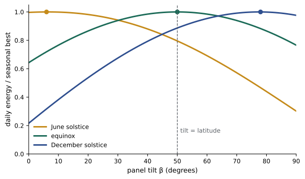
- This is greatest when \(\beta = \varphi = 50°\). A horizontal panel receives \(\cos 50° = 0.64\) of the optimum.
Answer: At the equinox the best tilt equals the latitude, 50°, and a flat panel collects only 64% as much. Repeating the calculation numerically for the solstices (where the sun's declination is ±23.45°) gives best tilts of about 6° in June and 78° in December at this latitude; a panel fixed at the latitude angle collects about 80% of the June optimum and 89% of the December optimum. Real designs also account for the atmosphere, clouds, snow shedding and the electricity price at different times of year.
Case study 3: laminar flow in a pipe
For slow, steady flow of a viscous fluid along a straight pipe of radius R, the velocity u is along the axis and depends only on the radius r. The Navier-Stokes equations (Lesson 10) reduce to a balance between the pressure gradient G = −dp/dx (positive when pressure falls along the pipe) and viscous friction, written with the cylindrical Laplacian (Lesson 9):
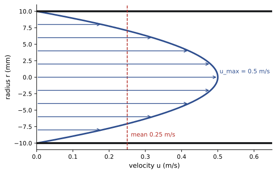
Integrating twice, with u finite on the axis and zero at the wall (no slip), gives the parabolic Poiseuille profile:
The flow rate is the flux of velocity through the cross-section, a double integral in polar coordinates (Lesson 5): \(Q = \int_0^{2\pi}\int_0^R u\,r\,dr\,d\theta = \dfrac{\pi GR^4}{8\mu}\). The mean velocity is half the maximum, and the wall shear stress is \(\tau_w = \mu|du/dr|_{r=R} = GR/2\).
Worked problem
Oil in a lubrication line
Oil (μ = 0.10 Pa·s, ρ = 900 kg/m³) flows through a tube of radius 10 mm with a pressure drop of 2.0 kPa per meter. Find the maximum velocity, flow rate, wall shear stress and Reynolds number.
Show solution
- \(u_{max} = GR^2/(4\mu) = 2000 \times 10^{-4}/0.4 = 0.50\) m/s.
- \(Q = \pi R^2u_{max}/2 = \pi \times 10^{-4} \times 0.25 = 7.85 \times 10^{-5}\) m³/s, or 0.079 L/s.
- \(\tau_w = GR/2 = 2000 \times 0.01/2 = 10\) Pa.
- Reynolds number \(Re = \rho\bar{u}D/\mu = 900 \times 0.25 \times 0.02/0.10 = 45\).
Answer: u_max = 0.50 m/s, Q = 0.079 L/s and τ_w = 10 Pa. With Re = 45, far below about 2000, the flow is indeed laminar and the model applies. The R⁴ in the flow rate is striking: a 10% narrower pipe carries 34% less flow at the same pressure drop, which is why small deposits in pipes and arteries matter so much.
Common threads
The three studies used different tools but the same approach:
- Describe the geometry with suitable coordinates: heights on a facade, vectors toward the sun, radius in a pipe.
- Express the physics as fields (pressure, light flux, velocity) and the quantities wanted as integrals, derivatives or extremes of those fields.
- Exploit symmetry to reduce dimensions: the pipe problem collapsed from three dimensions to one.
- Solve in closed form where possible, and check numerically, or the reverse.
- Check limits and validity: the Reynolds number for laminar flow, the uniform-pressure estimate for wind, the atmosphere neglected for sunlight.
- Interpret: a resultant height for the foundation designer, a tilt for the installer, a flow rate for the lubrication system.
The course project
Choose one of the following problems, or propose your own of similar scope with your instructor's approval, and prepare a technical report with your formulation, analysis, results (analytical and numerical) and interpretation.
- Project A: Terrain and earthworks. Obtain or construct a contour map of a site. Model the surface as a function of two variables, find slopes and drainage directions from the gradient, locate high and low points, and compute the cut and fill volumes needed to level a building pad by double integration.
- Project B: Optimal design. Choose a component (a tank, beam, duct, heat sink or panel layout) with at least two design variables and one constraint. Formulate the objective, solve with Lagrange multipliers and numerically, interpret the multiplier, and examine how the optimum changes if the objective or constraint changes.
- Project C: Flow field. Construct a two-dimensional potential flow from sources, sinks, vortices and uniform flow to model a practical situation (flow past a bridge pier, toward a well field or around a building). Plot streamlines, compute pressures with Bernoulli's equation, verify incompressibility and irrotationality, and discuss where the ideal-flow model fails.
- Project D: Field computation. Solve Laplace's equation numerically for an electrostatic, heat conduction or seepage problem in a non-rectangular region. Check your solver against an exact solution (a coaxial cable or a pipe wall), then compute a quantity of engineering interest such as capacitance, heat loss or seepage flow.
Every report should state the physical laws and assumptions, show the coordinate system and any changes of variables, verify results by an independent method, discuss sensitivity to uncertain inputs and conclude with clear engineering recommendations.
Working with software
Engineering software for structures, fluids, heat and electromagnetics is built on the mathematics of this course: finite element and finite volume programs integrate over elements, apply the divergence theorem to each cell and solve the resulting equations; optimization tools compute gradients and Hessians; geographic and surveying software works with surfaces and contours. Using such tools well requires knowing what they compute, choosing meshes and tolerances sensibly, and checking results against hand calculations like those in this lesson.
Looking ahead
Multivariable calculus is the language of the engineering sciences. Fluid mechanics, heat transfer, electromagnetics, solid mechanics and geotechnics all express their laws with gradients, divergences, curls and integrals over regions and surfaces. Differential equations (MATH-201) solve the resulting equations in simple cases, and numerical methods (MATH-300) solve them in general. Statistics (STAT-235) uses multiple integrals for joint distributions. The geometric intuition built here, of fields, flux and circulation, will make each of those subjects easier to understand.
Common mistakes
MistakeAssuming a uniform load where it varies with position.
InsteadIntegrate the actual distribution; it changes both the total and where it acts.
MistakeForgetting to clip negative values of s · n when the sun is behind a panel.
InsteadOnly positive incidence collects energy; integrate max(0, s · n).
MistakeApplying the Poiseuille formula to turbulent flow.
InsteadCheck that the Reynolds number is below about 2000.
MistakeIgnoring symmetry and solving a harder problem than necessary.
InsteadUse coordinates that match the geometry to reduce the number of variables.
MistakeReporting a numerical result without a check.
InsteadCompare with a closed-form special case or a simpler estimate.
Summary and key terms
- Wind load is an integral of a height-dependent pressure; for a power-law profile the resultant acts above mid-height.
- Solar energy on a panel is the time integral of a flux, IA s · n.
- At the equinox, the best fixed tilt equals the latitude; the best tilt varies with the season.
- Laminar pipe flow has a parabolic profile; Q = πGR⁴/(8μ) and τ_w = GR/2.
- Symmetry and well-chosen coordinates reduce problems to fewer variables.
- Closed-form results and numerical results should check each other.
- The course project applies the tools of the course to a design or analysis problem of your choice.
- Power-law wind profile
- A model of wind speed increasing as a power of height.
- Overturning moment
- The moment of lateral loads about the base of a structure.
- Angle of incidence
- The angle between incoming radiation and the surface normal.
- Hour angle
- The angle the Earth has turned since solar noon, 15° per hour.
- Declination
- The angle of the sun north or south of the equator, ±23.45° at the solstices.
- Poiseuille flow
- Steady laminar flow in a pipe, with a parabolic velocity profile.
- Wall shear stress
- The friction stress exerted by a fluid on a wall.
- Reynolds number
- ρūD/μ, the ratio of inertial to viscous effects, which indicates laminar or turbulent flow.
Practice problems
Work each problem on paper first, then reveal the answer to check.
For a uniform wind pressure on a face of height H, where does the resultant act?
Show answer
At mid-height, H/2.
For the power-law profile with α = 0.2, what fraction of the height is the resultant?
Show answer
(1 + 2α)/(2 + 2α) = 1.4/2.4 = 0.583.
By what factor does the wind force change if v₁₀ rises from 30 to 36 m/s?
Show answer
(36/30)² = 1.44.
Find s · n for a horizontal panel at noon on the equinox at latitude 45°.
Show answer
cos 45° = 0.707.
At latitude 45°, what fraction of the equinox optimum does a vertical south-facing panel collect?
Show answer
cos(45° − 90°) = 0.707.
Why is the June optimum tilt small at latitude 50°?
Show answer
The sun is high in the sky in summer, so a nearly flat panel faces it best.
In the oil example, what is the velocity at r = 5 mm?
Show answer
0.5(1 − 0.25) = 0.375 m/s.
If the pipe radius doubles at the same pressure gradient, how does Q change?
Show answer
It rises 16 times.
Find the flow rate for water (μ = 0.001 Pa·s) in a 1 mm radius tube with G = 100 Pa/m.
Show answer
π(100)(10⁻¹²)/(0.008) = 3.9 × 10⁻⁸ m³/s.
Check the Reynolds number for that water flow.
Show answer
ū = Q/(πR²) = 0.0125 m/s; Re = 1000 × 0.0125 × 0.002/0.001 = 25: laminar.
Lesson quiz · 5 questions
Score 60% or more to complete this lesson.
Create a free account to save your progress, take quizzes and earn a certificate.