
MATH-201 · Lesson 5 of 5 · 32 min
Systems of ODEs
Real systems rarely have just one moving part. Two tanks exchange fluid; the floors of a building sway against each other; a vehicle body bounces on its suspension while its wheels bounce on the tires; a chemical reaction consumes one species while producing another; predators and prey rise and fall together. Each needs several unknowns that depend on each other, governed by a system of differential equations.
This final chapter shows how to write such systems in matrix form, solve linear constant-coefficient systems with eigenvalues and eigenvectors (from MATH-125), interpret the results physically as decay modes and vibration modes, picture behavior with phase portraits, and solve systems numerically, including nonlinear ones, with a few lines of Python.
Systems in matrix form
A linear system of first-order equations with constant coefficients is written
where A is a constant square matrix. Every higher-order equation can be rewritten this way, which is how numerical solvers handle them: introduce the derivatives as new unknowns.
Worked problem
From second order to a system
Write \(y'' + 3y' + 2y = 0\) as a first-order system.
Show solution
- Let \(x_1 = y\) and \(x_2 = y'\). Then \(x_1' = x_2\), and from the equation \(x_2' = y'' = -2x_1 - 3x_2\).
- \[\begin{pmatrix} x_1 \\ x_2 \end{pmatrix}' = \begin{pmatrix} 0 & 1 \\ -2 & -3 \end{pmatrix}\begin{pmatrix} x_1 \\ x_2 \end{pmatrix}\]
Answer: The eigenvalues of this matrix are −1 and −2, the same as the characteristic roots in Lesson 4: the two descriptions are equivalent
Solving x′ = Ax with eigenvalues
Try \(\mathbf{x} = \mathbf{v}e^{\lambda t}\), a fixed vector times an exponential. Substituting gives \(\lambda\mathbf{v}e^{\lambda t} = A\mathbf{v}e^{\lambda t}\), so
The exponents are the eigenvalues of A and the vectors are its eigenvectors. For an n × n matrix with n independent eigenvectors, the general solution is a combination of these modes:
Each mode is a fixed pattern (the eigenvector) that grows or decays at its own rate (the eigenvalue). The initial condition decides how much of each mode is present.
Worked problem
Two interconnected tanks
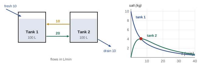
Two 100 L tanks are connected as shown. Fresh water enters tank 1 at 10 L/min; 20 L/min flows from tank 1 to tank 2; 10 L/min flows back from tank 2 to tank 1; 10 L/min drains from tank 2. Initially tank 1 holds 10 kg of dissolved salt and tank 2 none. Find the salt in each tank over time.
Show solution
- Salt balances (concentration = salt/100): \(x_1' = -\tfrac{20}{100}x_1 + \tfrac{10}{100}x_2\) and \(x_2' = \tfrac{20}{100}x_1 - \tfrac{20}{100}x_2\) (10 back plus 10 drained).
- \[A = \begin{pmatrix} -0.2 & 0.1 \\ 0.2 & -0.2 \end{pmatrix}\]
- Eigenvalues: \(\det(A - \lambda I) = (\lambda + 0.2)^2 - 0.02 = 0\), so \(\lambda = -0.2 \pm 0.1414\): \(\lambda_1 = -0.0586\), \(\lambda_2 = -0.3414\).
- Eigenvectors: \(\mathbf{v}_1 = (1, \sqrt{2})\), \(\mathbf{v}_2 = (1, -\sqrt{2})\).
- Initial condition (10, 0): \(C_1 + C_2 = 10\) and \(\sqrt{2}(C_1 - C_2) = 0\), so \(C_1 = C_2 = 5\).
- \[x_1 = 5e^{-0.0586t} + 5e^{-0.3414t}, \qquad x_2 = 7.07\left(e^{-0.0586t} - e^{-0.3414t}\right)\]
Answer: Both decay to zero (all eigenvalues negative). Tank 2 peaks at about 4.07 kg after 6.2 minutes, found by setting x₂′ = 0. The slow mode (time constant 1/0.0586 = 17 min) controls how long the system takes to flush; the fast mode (2.9 min) is the initial redistribution between tanks
Vibration modes
For undamped mechanical systems, Newton's law gives a second-order matrix equation \(M\ddot{\mathbf{x}} + K\mathbf{x} = \mathbf{0}\), with a mass matrix M and a stiffness matrix K. Trying \(\mathbf{x} = \boldsymbol{\phi}\cos\omega t\) gives the eigenvalue problem
Each eigenvalue \(\omega^2\) gives a natural frequency, and each eigenvector \(\boldsymbol{\phi}\) a mode shape: the pattern in which all the masses move together at that frequency. A structure with n degrees of freedom has n natural frequencies and n modes. Earthquake engineers design buildings by examining these modes; the first (lowest) mode usually dominates the response.
Worked problem
A two-story building
Model a two-story frame as two floor masses of 20 t each, with story stiffness k = 8 MN/m for each story. Find the natural frequencies and mode shapes.
Show solution
- Floor 1 is connected to the ground and to floor 2; floor 2 only to floor 1. With m = 20 000 kg:
- \[M = m\begin{pmatrix} 1 & 0 \\ 0 & 1 \end{pmatrix}, \qquad K = k\begin{pmatrix} 2 & -1 \\ -1 & 1 \end{pmatrix}\]
- With \(\mu = \omega^2 m/k\): \(\det\begin{pmatrix} 2 - \mu & -1 \\ -1 & 1 - \mu \end{pmatrix} = \mu^2 - 3\mu + 1 = 0\), so \(\mu = (3 \mp \sqrt{5})/2 = 0.382, 2.618\).
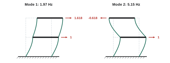
- \(k/m = 400\) s⁻², so \(\omega_1 = \sqrt{0.382 \times 400} = 12.4\) rad/s (1.97 Hz) and \(\omega_2 = \sqrt{2.618 \times 400} = 32.4\) rad/s (5.15 Hz).
- Mode shapes from the first row, \((2 - \mu)\phi_1 = \phi_2\): mode 1: \((1, 1.618)\); mode 2: \((1, -0.618)\).
Answer: Mode 1 at 1.97 Hz: both floors sway the same way, the top more. Mode 2 at 5.15 Hz: the floors move in opposite directions. A numerical eigenvalue solver gives the same values
Phase portraits and stability
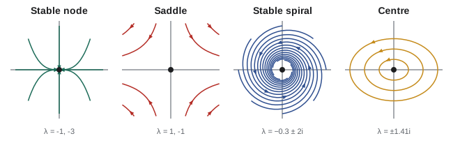
For a two-dimensional system, plot \(x_2\) against \(x_1\) instead of each against time. Each solution traces a curve, a trajectory, in this phase plane, and a set of trajectories is a phase portrait. The eigenvalues of A determine its shape around the equilibrium at the origin:
- Both eigenvalues real and negative: a stable node; all trajectories flow into the origin.
- Real with opposite signs: a saddle; almost all trajectories eventually run away. Unstable.
- Complex with negative real part: a stable spiral; trajectories spiral in (a damped oscillation).
- Purely imaginary: a center; closed orbits (an undamped oscillation).
- Any eigenvalue with positive real part: unstable.
Worked problem
Classifying equilibria
Classify the origin for \(\mathbf{x}' = A\mathbf{x}\) with (a) \(A = \begin{pmatrix} 0 & 1 \\ -2 & -3 \end{pmatrix}\); (b) \(A = \begin{pmatrix} 1 & 2 \\ 2 & 1 \end{pmatrix}\); (c) \(A = \begin{pmatrix} 0 & 1 \\ -100 & -6 \end{pmatrix}\).
Show solution
- (a) Eigenvalues −1, −2: stable node (the overdamped system from earlier).
- (b) \((1 - \lambda)^2 = 4\): \(\lambda = 3, -1\). Opposite signs: saddle, unstable.
- (c) \(\lambda^2 + 6\lambda + 100 = 0\): \(\lambda = -3 \pm 9.54i\). Stable spiral: the quarter-car suspension from Lesson 4.
Answer: (a) stable node; (b) saddle (unstable); (c) stable spiral. For 2 × 2 systems a shortcut works: with trace T and determinant D, stability needs T < 0 and D > 0
Numerical solution
Most real systems, especially nonlinear ones, have no closed-form solution. Numerical solvers step them forward in time with much more accurate versions of Euler's method (ENCM-100). In Python, scipy.integrate.solve_ivp does this for any system written as a function returning \(\mathbf{x}'\).
import numpy as np
from scipy.integrate import solve_ivp

A = np.array([[-0.2, 0.1],
              [ 0.2, -0.2]])

def rates(t, x):
    return A @ x

sol = solve_ivp(rates, [0, 30], [10, 0], dense_output=True, rtol=1e-8)
x1, x2 = sol.sol(10)
print(f"After 10 min: tank 1 = {x1:.3f} kg, tank 2 = {x2:.3f} kg")
Output: After 10 min: tank 1 = 2.948 kg, tank 2 = 3.704 kg, matching the eigenvalue solution. Changing the model to a nonlinear one, or to 50 tanks, changes only the rates function.
A nonlinear system: predators and prey
The Lotka-Volterra model describes two interacting populations, prey x and predators y:
Prey grow on their own and are eaten; predators die off on their own and grow by eating. The same structure appears in ecology, in some chemical reaction networks and in economics. Linearizing near an equilibrium (using the matrix of partial derivatives, the Jacobian, from MATH-209) shows its local behavior.
Worked problem
Equilibrium of a predator-prey system
For \(x' = 0.4x - 0.02xy\), \(y' = -0.3y + 0.01xy\), find the coexistence equilibrium and its type.
Show solution
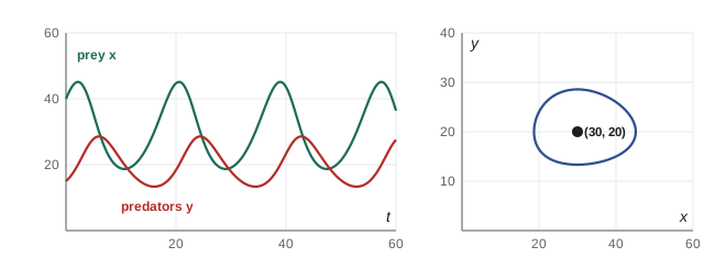
- Set both rates to zero with \(x, y > 0\): \(0.4 = 0.02y\) gives \(y = 20\); \(0.3 = 0.01x\) gives \(x = 30\).
- Jacobian at (30, 20): \(\begin{pmatrix} 0.4 - 0.02y & -0.02x \\ 0.01y & -0.3 + 0.01x \end{pmatrix} = \begin{pmatrix} 0 & -0.6 \\ 0.2 & 0 \end{pmatrix}\).
- Eigenvalues: \(\lambda^2 + 0.12 = 0\), \(\lambda = \pm 0.346i\): a center.
Answer: Equilibrium (30 prey, 20 predators), surrounded by closed orbits: the populations cycle with a period of about 2π/0.346 ≈ 18 time units, predators lagging prey
This is where the course ends and much of engineering analysis begins. The finite element programs that analyze structures, the circuit simulators that design electronics, the process simulators that run chemical plants and the climate and reservoir models that inform policy all solve very large systems of differential equations. Every one of them relies on the ideas here: linearity and superposition, modes and eigenvalues, stability, and careful numerical solution checked against cases you can solve by hand.
Common mistakes
MistakeGetting the matrix entries from a mass balance with the wrong signs.
InsteadOutflows from a tank are negative on its diagonal; inflows from another tank are positive off-diagonal. Check that each column sums sensibly for closed systems.
MistakeFitting initial conditions to each mode separately.
InsteadSolve for all constants together from x(0) = C₁v₁ + C₂v₂ + ….
MistakeConfusing ω² (the eigenvalue) with ω in vibration problems.
InsteadKφ = ω²Mφ: take the square root to get rad/s, then divide by 2π for Hz.
MistakeJudging stability from the matrix entries rather than eigenvalues.
InsteadCompute the eigenvalues (or for 2 × 2, check trace < 0 and determinant > 0).
MistakeTrusting a numerical solution without any check.
InsteadVerify on a case with a known solution, and check that tightening the tolerance does not change the answer.
MistakeAssuming linear results hold far from equilibrium in nonlinear systems.
InsteadLinearization describes behavior only near the equilibrium; use numerical solution for large motions.
Summary and key terms
- Linear systems are written x′ = Ax + f(t); any higher-order ODE can be rewritten as a first-order system.
- Solutions of x′ = Ax are combinations of modes vᵢe^{λᵢt}, from the eigenvalues and eigenvectors of A.
- The eigenvalue nearest zero (the dominant mode) sets the settling time of a stable system.
- Undamped vibration: Kφ = ω²Mφ gives natural frequencies and mode shapes; n degrees of freedom give n modes.
- Phase portraits: stable node, saddle, stable spiral and center correspond to eigenvalue cases; stability needs all real parts negative.
- Nonlinear systems are linearized with the Jacobian near equilibria and solved numerically, for example with scipy's solve_ivp.
- System of ODEs
- Several differential equations for several coupled unknowns.
- Coefficient matrix
- The constant matrix A in x′ = Ax.
- Mode
- A solution of fixed shape (an eigenvector) varying as e^{λt}.
- Dominant mode
- The slowest-decaying mode, which controls settling time.
- Mass and stiffness matrices
- M and K in Mẍ + Kx = 0 for a multi-degree-of-freedom system.
- Mode shape
- The pattern of relative motion at one natural frequency.
- Phase plane
- The plane of the state variables in which trajectories are drawn.
- Equilibrium point
- A state where all rates are zero.
- Saddle
- An unstable equilibrium with eigenvalues of opposite sign.
- Jacobian matrix
- The matrix of partial derivatives used to linearize a nonlinear system.
Practice problems
Work each problem on paper first, then reveal the answer to check.
Write y″′ + 2y″ − y′ + 5y = 0 as a first-order system.
Show answer
x₁ = y, x₂ = y′, x₃ = y″: x₁′ = x₂, x₂′ = x₃, x₃′ = −5x₁ + x₂ − 2x₃.
Solve x′ = Ax with A = [[−1, 0], [0, −3]] and x(0) = (2, 5).
Show answer
Uncoupled: x₁ = 2e^{−t}, x₂ = 5e^{−3t}.
Find the eigenvalues and eigenvectors of A = [[−3, 1], [1, −3]].
Show answer
λ = −2 with v = (1, 1); λ = −4 with v = (1, −1).
For that matrix, solve with x(0) = (4, 0).
Show answer
C₁ = C₂ = 2: x₁ = 2e^{−2t} + 2e^{−4t}, x₂ = 2e^{−2t} − 2e^{−4t}.
In the two-tank example, what is the time constant of the dominant mode, and roughly how long until the total salt is under 1% of the original?
Show answer
τ = 1/0.0586 = 17.1 min. The slow mode dominates; about ln(100) × 17.1 ≈ 79 min (slightly less because the fast mode also contributes at first).
Two equal masses m = 5 kg are joined to each other and to two walls by three springs of k = 500 N/m (wall–m–m–wall). Find the natural frequencies.
Show answer
K = k[[2, −1], [−1, 2]], ω² = k/m and 3k/m: ω₁ = 10 rad/s (in-phase mode), ω₂ = 17.3 rad/s (out-of-phase mode).
In the two-story building, if the story stiffness doubled, what would happen to the frequencies?
Show answer
They scale with √k: both increase by √2, to 2.78 Hz and 7.28 Hz. Mode shapes are unchanged.
Classify the origin for A = [[−1, −4], [1, −1]].
Show answer
λ² + 2λ + 5 = 0, λ = −1 ± 2i: stable spiral.
Use the trace-determinant test on A = [[2, 1], [−3, −4]].
Show answer
T = −2, D = −8 + 3 = −5 < 0: saddle, unstable.
For the predator-prey model, what happens to the equilibrium prey population if the predator death rate c doubles to 0.6?
Show answer
x* = c/d = 60: twice as many prey at equilibrium. (Predators y* = a/b = 20 is unchanged.)
Lesson quiz · 5 questions
Score 60% or more to complete this lesson.
Create a free account to save your progress, take quizzes and earn a certificate.