Matrix algebra

In Lesson 2 a matrix was a convenient table for bookkeeping. In this chapter it becomes an object in its own right, with its own arithmetic. Matrices can be added, multiplied and (sometimes) inverted, and once you can do that, a system of a thousand equations can be written as the single line \(A\mathbf{x} = \mathbf{b}\) and reasoned about as easily as \(ax = b\).

Matrices also act. Multiplying a vector by a matrix rotates, stretches, shears or projects it. This view of a matrix as a transformation is behind computer graphics, robot kinematics, coordinate changes in stress analysis and the stiffness method in structural engineering. By the end of this chapter you will be able to set up and solve a small stiffness model yourself.

Matrices and notation

An \(m \times n\) matrix is a rectangular array with \(m\) rows and \(n\) columns. The entry in row \(i\), column \(j\) is written \(a_{ij}\). Rows come first, always: a 2×3 matrix has 2 rows and 3 columns.

A matrix with one column is a column vector, and that is how vectors are written in linear algebra from now on. A square matrix has as many rows as columns. Its main diagonal runs from top left to bottom right. Some special square matrices have names:

• The identity matrix \(I\) has 1s on the diagonal and 0s elsewhere. It plays the role of the number 1.
• A diagonal matrix has non-zero entries only on the diagonal.
• An upper triangular matrix has zeros below the diagonal, like the echelon forms in Lesson 2.
• A symmetric matrix equals its own transpose: \(a_{ij} = a_{ji}\).

Addition and scalar multiplication

Matrices of the same size add entry by entry, and a scalar multiplies every entry. These operations behave just like ordinary arithmetic: \(A + B = B + A\), \(c(A + B) = cA + cB\), and so on.

You cannot add matrices of different sizes. A 2×3 plus a 3×2 is undefined.

Multiplying a matrix by a vector

The product \(A\mathbf{x}\) can be read in two ways, and both are worth knowing.

By rows: each entry of \(A\mathbf{x}\) is the dot product of a row of \(A\) with \(\mathbf{x}\). This is how you compute it, and it is why \(A\mathbf{x} = \mathbf{b}\) is the same as the system of equations: row \(i\) dotted with \(\mathbf{x}\) equals \(b_i\).

By columns: \(A\mathbf{x}\) is a combination of the columns of \(A\), weighted by the entries of \(\mathbf{x}\):

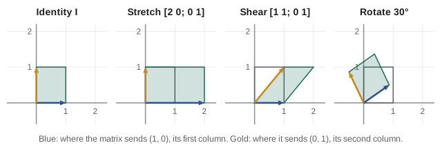
The column view explains what solving \(A\mathbf{x} = \mathbf{b}\) means: finding the amounts of each column that combine to give \(\mathbf{b}\). It also explains the transformation picture. The first column of \(A\) is where \(A\) sends \((1, 0)\), and the second column is where it sends \((0, 1)\). Knowing those two images tells you where every other vector goes.

Matrix multiplication

The product \(AB\) is defined when the number of columns of \(A\) equals the number of rows of \(B\). If \(A\) is \(m \times n\) and \(B\) is \(n \times p\), then \(AB\) is \(m \times p\). The entry in row \(i\), column \(j\) of \(AB\) is the dot product of row \(i\) of \(A\) with column \(j\) of \(B\):

A quick size check before you start: write the sizes side by side, \((m \times n)(n \times p)\). The inner numbers must match, and the outer numbers give the size of the answer.

Order matters

Matrix multiplication is not commutative. Usually \(AB \ne BA\), even when both are defined and the same size.

The transformation view explains why. \(AB\mathbf{x}\) means "apply \(B\) first, then \(A\)". Rotating then stretching is not the same as stretching then rotating. For instance, with \(R\) a 90° rotation and \(S\) a horizontal stretch by 2, \(SR = \begin{pmatrix} 0 & -2 \\ 1 & 0 \end{pmatrix}\) but \(RS = \begin{pmatrix} 0 & -1 \\ 2 & 0 \end{pmatrix}\).

Apart from commutativity, the familiar rules survive: \((AB)C = A(BC)\), \(A(B + C) = AB + AC\), and \(AI = IA = A\). Two other surprises: \(AB = 0\) is possible with neither \(A\) nor \(B\) zero, and \(AB = AC\) does not let you cancel \(A\) unless \(A\) is invertible.

The transpose

The transpose \(A^T\) swaps rows and columns: \((A^T)_{ij} = a_{ji}\). A 2×3 matrix has a 3×2 transpose. Its rules:

• \((A^T)^T = A\) and \((A + B)^T = A^T + B^T\).
• \((AB)^T = B^T A^T\). The order reverses, like taking off socks and shoes.
• The dot product is a matrix product: \(\mathbf{u}\cdot\mathbf{v} = \mathbf{u}^T\mathbf{v}\).

Symmetric matrices (\(A^T = A\)) are everywhere in engineering: stiffness matrices, stress tensors, inertia tensors, covariance matrices. For any matrix \(A\), the product \(A^TA\) is square and symmetric; it is the heart of least-squares curve fitting.

The inverse

For numbers, the solution of \(ax = b\) is \(x = a^{-1}b\), provided \(a \ne 0\). The matrix version is the inverse. A square matrix \(A\) is invertible if there is a matrix \(A^{-1}\) with

Then \(A\mathbf{x} = \mathbf{b}\) has the unique solution \(\mathbf{x} = A^{-1}\mathbf{b}\). A matrix without an inverse is called singular. Only square matrices can have inverses, and many square matrices do not, just as 0 has no reciprocal.

2×2 inverses

For a 2×2 matrix there is a formula worth memorizing:

Swap the diagonal entries, negate the off-diagonal ones, and divide by \(ad - bc\). That number is the determinant, the subject of Lesson 4. If it is zero, there is no inverse.

Larger inverses by Gauss–Jordan

For bigger matrices, write \(A\) and \(I\) side by side as \([A \mid I]\) and apply Gauss–Jordan elimination to the whole thing. When the left side becomes \(I\), the right side is \(A^{-1}\). If the left side develops a row of zeros, \(A\) is singular.

Inverse rules, and when not to use one

If \(A\) and \(B\) are invertible, then \((AB)^{-1} = B^{-1}A^{-1}\) (order reverses again) and \((A^T)^{-1} = (A^{-1})^T\).

In practice, engineers rarely compute an inverse to solve a system. Elimination solves \(A\mathbf{x} = \mathbf{b}\) with about a third of the work of finding \(A^{-1}\), and with less rounding error. Software factors \(A = LU\) (a lower triangular matrix times an upper triangular one, which is just elimination written down) and reuses the factors for each new right-hand side. The inverse is still essential as an idea: it tells you whether a unique solution exists and gives formulas such as \(\mathbf{x} = A^{-1}\mathbf{b}\) for analysis.

Application: a stiffness model

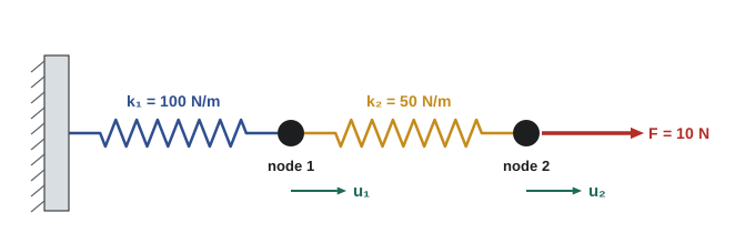
The stiffness method, the basis of structural analysis software and the finite-element method, writes the equilibrium of a structure as \(K\mathbf{u} = \mathbf{F}\). Here \(\mathbf{u}\) lists the unknown displacements of the nodes, \(\mathbf{F}\) the applied forces, and \(K\) is the stiffness matrix.

Notice that \(K\) is symmetric, as stiffness matrices always are. If the wall were removed, \(K\) would become \(\begin{pmatrix} k_2 & -k_2 \\ -k_2 & k_2 \end{pmatrix}\), which is singular: an unsupported structure can slide freely, so there is no unique displacement. Software that reports a "singular stiffness matrix" is telling you the model is missing a support.