
ELE-360 · Lesson 9 of 12 · 24 min
Transmission lines
In the cabinet at each intersection, the TLR-1 radio sits on a DIN rail, and a coaxial cable climbs inside the pole and out along the mast arm to an antenna about 12 m away. At 915 MHz that cable is about 43 wavelengths long. A signal entering one end does not appear at the other end instantly; it travels as a wave, taking about 50 ns, losing some of its power on the way, and if the antenna at the far end does not match the cable, part of it bounces back. Circuit theory, with its assumption that a wire has the same voltage along its whole length, cannot describe this. Transmission-line theory can, and it does so without solving Maxwell's equations in three dimensions: it describes the line by a few parameters per unit length and treats the voltage and current along it as waves.
Transmission-line theory is the most practically useful part of electromagnetics for an electronics engineer. It applies to coaxial cables, twisted pairs, printed-circuit traces, power lines and the leads of a fast oscilloscope probe. Its results, characteristic impedance, reflection coefficient, standing-wave ratio and return loss, appear on every radio datasheet. This lesson builds the model and the traveling-wave solution, computes the parameters of the TLR-1 feeder from its geometry, and shows how loss and mismatch affect the power that reaches the antenna.
The distributed model
A transmission line is two conductors, such as the center and shield of a coaxial cable or a trace and its ground plane, running parallel for a long distance. Divide it into short sections of length Δz, each much shorter than a wavelength. Each section has a series inductance L′Δz, from the magnetic flux between the conductors, and a series resistance R′Δz, from the conductors' losses. Across the section there is a shunt capacitance C′Δz, from the electric flux between the conductors, and a shunt conductance G′Δz, from the dielectric's losses. The four per-unit-length parameters R′, L′, G′ and C′ capture everything the fields do, provided the fields are transverse to the line, as they are in coaxial cable and very nearly so on a printed-circuit trace.
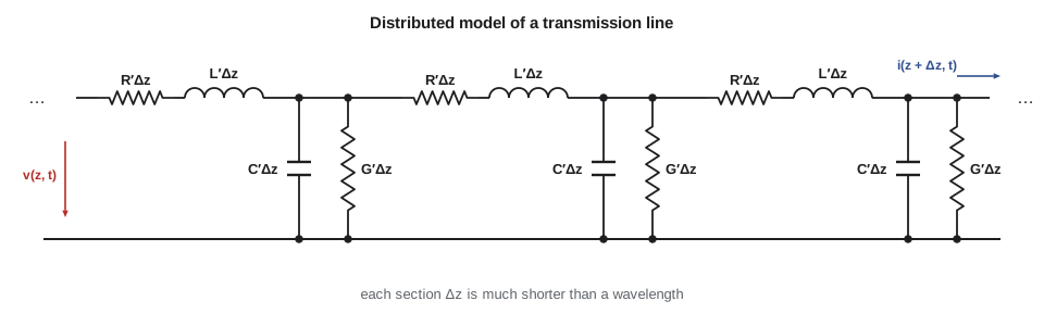
Applying Kirchhoff's laws to one section and letting Δz shrink to zero gives the telegrapher's equations, named for their nineteenth-century use in describing signals on long telegraph and undersea cables. In phasor form they say that the rate of change of voltage along the line is set by the series impedance per unit length times the current, and the rate of change of current by the shunt admittance per unit length times the voltage. Combining them gives a wave equation for V(z).
Traveling waves and characteristic impedance
The solution is a pair of traveling waves, V(z) = V⁺e^{−γz} + V⁻e^{+γz}, with propagation constant γ = α + jβ = √((R′ + jωL′)(G′ + jωC′)). The forward wave V⁺ travels toward +z and the reflected wave V⁻ toward −z. Each wave has a current related to its voltage by the characteristic impedance Z₀ = √((R′ + jωL′)/(G′ + jωC′)): I⁺ = V⁺/Z₀ and I⁻ = −V⁻/Z₀. The characteristic impedance is the impedance a single traveling wave sees. It is not a resistance you can measure with an ohmmeter, and it does not depend on the length of the line. It is the line's equivalent of the intrinsic impedance η of lesson 7, and the analogy is exact: on a coaxial line, the voltage is the integral of the radial E between the conductors and the current is the circulation of the circling H.
For a lossless line, or a low-loss one at radio frequencies where ωL′ ≫ R′ and ωC′ ≫ G′, Z₀ is real and equal to √(L′/C′), and the phase velocity is 1/√(L′C′). For a line whose fields lie entirely in one dielectric, such as a coaxial cable, L′C′ = με, so the phase velocity is c/√ε_r, the same as a plane wave in that dielectric. The ratio v_p/c is the velocity factor printed on cable datasheets: about 0.66 for solid polyethylene, 0.8 to 0.88 for foamed polyethylene and about 0.7 for PTFE.
| Line | Characteristic impedance (lossless) | Notes |
|---|---|---|
| Coaxial, radii a < b | Z₀ = (60/√ε_r) ln(b/a) Ω | 50 Ω for radio, 75 Ω for video and cable television |
| Two-wire, radius a, spacing D | Z₀ = (120/√ε_r) arccosh(D/2a) Ω | Twin-lead about 300 Ω; twisted pair about 100 Ω |
| Microstrip, width w over height h | Curve fits (lesson 11) | Depends on w/h and ε_r; 50 Ω on 1.6 mm FR-4 is about 3 mm wide |
| Parallel plates, width w, spacing d | Z₀ = η d/w | Valid for w ≫ d |
The TLR-1 feeder
Amara compares two cables for the cabinet antenna run. The first is a thin flexible 50 Ω cable of the common type with a 0.9 mm center conductor and solid polyethylene dielectric 2.95 mm across. The second is a thicker low-loss cable, about 10 mm across, with a 2.74 mm center conductor and a foamed polyethylene dielectric about 7.2 mm across with an effective ε_r of about 1.38. From the geometry alone, using lessons 3 and 4 for C′ and L′ and the skin-effect surface resistance of lesson 7 for R′, she computes Z₀, velocity and loss for each. Real cables have stranded or copper-clad steel center conductors and braided shields whose loss is higher than the smooth-copper model predicts, so she compares her figures with the manufacturers' published attenuation, which datasheets give in decibels per 100 m or per 100 ft at a list of frequencies.
import math, cmath
eps0, mu0, c = 8.854e-12, 4e-7 * math.pi, 2.998e8
f = 915e6; w = 2 * math.pi * f
Rs = math.sqrt(math.pi * f * mu0 / 5.8e7)        # copper surface resistance at 915 MHz
cables = (("thin 50 ohm (solid PE)", 0.45e-3, 1.475e-3, 2.25, 2e-4),
          ("low-loss 50 ohm (foam PE)", 1.37e-3, 3.62e-3, 1.38, 1e-4))
for name, a, b, er, tand in cables:
    Lp = mu0 / (2 * math.pi) * math.log(b / a)
    Cp = 2 * math.pi * eps0 * er / math.log(b / a)
    Z0 = math.sqrt(Lp / Cp); v = 1 / math.sqrt(Lp * Cp)
    Rp = Rs / (2 * math.pi) * (1 / a + 1 / b); Gp = w * Cp * tand
    ac, ad = Rp / (2 * Z0), Gp * Z0 / 2
    print(f"{name}: Z0 = {Z0:.1f} ohm, L' = {Lp*1e9:.0f} nH/m, C' = {Cp*1e12:.1f} pF/m, v = {v/c:.3f} c")
    print(f"   R' = {Rp:.2f} ohm/m, conductor {ac*8.686:.3f} dB/m + dielectric {ad*8.686:.3f} dB/m; 12 m = {(ac + ad)*8.686*12:.2f} dB, delay {12/v*1e9:.0f} ns")
# exact propagation constant and Z0 from R', L', G', C' for the low-loss cable
a, b, er, tand = cables[1][1:]
Lp = mu0 / (2 * math.pi) * math.log(b / a); Cp = 2 * math.pi * eps0 * er / math.log(b / a)
Z = Rs / (2 * math.pi) * (1 / a + 1 / b) + 1j * w * Lp; Y = w * Cp * tand + 1j * w * Cp
print(f"exact: Z0 = {cmath.sqrt(Z / Y).real:.2f} {cmath.sqrt(Z / Y).imag:+.2f}j ohm, alpha = {cmath.sqrt(Z * Y).real*8.686:.3f} dB/m")
# mismatch at the antenna
for vswr in (1.2, 1.5, 2.0, 3.0):
    G = (vswr - 1) / (vswr + 1)
    print(f"VSWR {vswr}: |Gamma| = {G:.3f}, return loss {-20*math.log10(G):5.1f} dB, mismatch loss {-10*math.log10(1 - G*G):.2f} dB")
# a lossy cable hides a bad antenna: the reflection is attenuated twice
for loss in (1.45, 4.30):
    G = 0.5
print(f"antenna |Gamma| = 0.5 behind {loss:.2f} dB of cable: |Gamma| at the radio {G * 10**(-2*loss/20):.3f}, return loss {-20*math.log10(G) + 2*loss:.1f} dB")thin 50 ohm (solid PE): Z0 = 47.5 ohm, L' = 237 nH/m, C' = 105.4 pF/m, v = 0.667 c R' = 3.64 ohm/m, conductor 0.333 dB/m + dielectric 0.025 dB/m; 12 m = 4.30 dB, delay 60 ns low-loss 50 ohm (foam PE): Z0 = 49.6 ohm, L' = 194 nH/m, C' = 79.0 pF/m, v = 0.851 c R' = 1.26 ohm/m, conductor 0.111 dB/m + dielectric 0.010 dB/m; 12 m = 1.45 dB, delay 47 ns exact: Z0 = 49.59 -0.03j ohm, alpha = 0.120 dB/m VSWR 1.2: |Gamma| = 0.091, return loss 20.8 dB, mismatch loss 0.04 dB VSWR 1.5: |Gamma| = 0.200, return loss 14.0 dB, mismatch loss 0.18 dB VSWR 2.0: |Gamma| = 0.333, return loss 9.5 dB, mismatch loss 0.51 dB VSWR 3.0: |Gamma| = 0.500, return loss 6.0 dB, mismatch loss 1.25 dB antenna |Gamma| = 0.5 behind 1.45 dB of cable: |Gamma| at the radio 0.358, return loss 8.9 dB antenna |Gamma| = 0.5 behind 4.30 dB of cable: |Gamma| at the radio 0.186, return loss 14.6 dB
The thin cable comes out at 47.5 Ω with a velocity factor of 0.667, 105 pF/m and an ideal-copper loss of about 0.36 dB/m at 915 MHz, or 4.3 dB for 12 m; manufacturers list somewhat more, around 0.5 to 0.6 dB/m, because of the stranded center and braided shield. The low-loss cable comes out at 49.6 Ω, a velocity factor of 0.85 and about 0.12 dB/m, or 1.45 dB for 12 m, close to published figures for this class of cable. The exact calculation from R′, L′, G′ and C′ confirms the low-loss approximations: Z₀ has a negligible imaginary part and α matches. Conductor loss dominates in both cables, which is why low-loss cables are thick. Since R′ grows as √f, cable loss in decibels grows roughly as the square root of frequency until dielectric loss, which grows as f, takes over at microwave frequencies.
Worked problem
Choosing the cabinet feeder
The ELE-350 link budget allowed 2 dB for the cabinet antenna feeder, including two connectors. The run is 12 m. Which cable fits, and what does each cost in link margin?
Show solution
- Thin cable: about 4.3 dB by the ideal model and about 6–7 dB by datasheet figures, plus connectors.
- Low-loss cable: about 1.45 dB plus roughly 0.1–0.2 dB per connector pair, about 1.7 dB in total.
- \[\Delta\text{margin} \approx 6.5 - 1.7 \approx 5\ \text{dB}\]
Answer: Only the low-loss cable meets the 2 dB allowance; the thin cable would cost about 5 dB of the cabinet link's margin, roughly what the external LNA of ELE-350 lesson 12 bought. Amara specifies the low-loss cable for the mast-arm run and keeps the thin flexible cable for a 0.5 m jumper inside the cabinet, where its loss is about a quarter of a decibel.
Terminations and the reflection coefficient
At the end of the line, at z = 0 say, a load Z_L forces V/I = Z_L. If Z_L = Z₀, a single forward wave already satisfies this and there is no reflection: the line is matched, and a matched line of any length looks like Z₀ from its input. Otherwise a reflected wave appears with voltage reflection coefficient Γ_L = V⁻/V⁺ = (Z_L − Z₀)/(Z_L + Z₀), the same form as the plane-wave formula of lesson 8. An open circuit gives Γ_L = +1, a short circuit −1 and a purely reactive load a reflection of magnitude 1 at some phase. A resistive load larger than Z₀ gives a positive Γ, smaller gives a negative one.
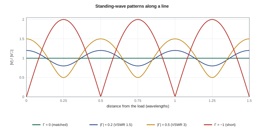
The forward and reflected waves interfere to form a standing-wave pattern along the line. The voltage magnitude oscillates between maxima of |V⁺|(1 + |Γ|) and minima of |V⁺|(1 − |Γ|), with maxima and minima a quarter wavelength apart. Their ratio is the voltage standing-wave ratio, VSWR, which runs from 1 for a matched line to infinity for an open or short. Return loss is how far below the forward wave the reflected wave is, in decibels: higher is better. Mismatch loss is the reduction in power delivered to the load because of the reflection. A VSWR of 1.5, a typical antenna specification, means |Γ| = 0.2, a return loss of 14 dB and a mismatch loss of only 0.18 dB; even a VSWR of 3 loses only 1.25 dB. Mismatch matters less for the power delivered than for what the reflected power does to the transmitter, and for the ripple it puts on a wideband system's response.
Loss, mismatch and what the radio sees
On a lossy line, the reflected wave is attenuated on its way back as well as the forward wave on its way out, so a reflection at the antenna is reduced at the radio by twice the cable loss. That improves the apparent return loss at the radio's end, which sounds good and is a trap: a long lossy cable makes even a broken antenna look reasonably matched. With the antenna at |Γ| = 0.5, a VSWR of 3, the low-loss feeder reduces the reflection seen at the radio to about 0.36, but the thin cable reduces it to about 0.19, which would pass a quick VSWR check while the antenna is far out of tune. The field rule follows: measure antenna match at the antenna end of the feeder, or use the time-domain methods of lesson 10 to look along the cable.
The radio's own output is designed for a 50 Ω load; a severe mismatch can reduce its output power, distort its spectrum or, in high-power transmitters, damage it. For the TLR-1's 100 mW the main concern is lost link margin, and the specification Amara writes is VSWR 1.5 or better across 902–928 MHz at the antenna connector, measured on a calibrated vector network analyzer. Lesson 10 shows how to transform impedances along the line and match a load that misses that target.
When a trace or cable is a transmission line
Lesson 6 gave a crude rule: anything longer than a tenth of a wavelength needs line theory. For digital signals, a better rule compares the line's one-way delay with the signal's rise time. If the delay is less than about a sixth of the rise time, reflections settle during the edge and the line can be treated as lumped. If it is longer, reflections appear as distinct steps and ringing, and the line must be terminated. On FR-4, signals travel at roughly 15 cm/ns on inner layers and somewhat faster on outer ones, so an edge of 1 ns makes a trace longer than about 2.5 cm a transmission line. The APS-2's codec clock, with edges of a few nanoseconds, runs 8 cm across the board and is at the borderline; lesson 11 adds a series termination resistor at its driver.
Common mistakes
MistakeMeasuring Z₀ with an ohmmeter.
InsteadZ₀ relates voltage to current in a traveling wave; a DC ohmmeter on an open line reads infinity.
MistakeAssuming a matched line's input impedance depends on length.
InsteadA line terminated in Z₀ looks like Z₀ at any length.
MistakeTrusting a good VSWR reading at the radio end of a long lossy cable.
InsteadCable loss attenuates the reflection twice; measure at the antenna end.
MistakeEquating VSWR with lost power.
InsteadVSWR 2 loses only 0.5 dB of delivered power; the reflected power matters mainly for the source and for ripple.
Summary and key terms
- A transmission line is described by R′, L′, G′ and C′ per unit length; the telegrapher's equations lead to traveling waves.
- Z₀ = √((R′ + jωL′)/(G′ + jωC′)) relates voltage and current in each wave; γ = α + jβ sets loss and phase.
- Lossless lines have Z₀ = √(L′/C′) and v_p = 1/√(L′C′); in a uniform dielectric v_p = c/√ε_r.
- Conductor loss grows as √f and dominates in cables at 915 MHz; dielectric loss grows as f.
- A load reflects Γ_L = (Z_L − Z₀)/(Z_L + Z₀); VSWR, return loss and mismatch loss describe the result.
- Reflections are attenuated twice by cable loss, so a lossy feeder hides a bad antenna.
- Characteristic impedance
- Z₀, the ratio of voltage to current in a single traveling wave on a line.
- Propagation constant
- γ = α + jβ, describing attenuation and phase change per unit length.
- Velocity factor
- The ratio of a line's phase velocity to the speed of light.
- Telegrapher's equations
- The coupled equations for voltage and current along a distributed line.
- Matched line
- A line terminated in its characteristic impedance, so there is no reflection.
- VSWR
- Voltage standing-wave ratio, the ratio of maximum to minimum voltage along a line.
- Return loss
- The ratio of forward to reflected power, in decibels.
- Mismatch loss
- The reduction in delivered power caused by reflection at a load.
Practice problems
Work each problem on paper first, then reveal the answer to check.
A lossless line has L′ = 250 nH/m and C′ = 100 pF/m. Find Z₀ and v_p.
Show answer
50 Ω; 2.0 × 10⁸ m/s (0.667c).
A 75 Ω cable feeds a 50 Ω load. Find Γ, VSWR and return loss.
Show answer
Γ = −0.2; VSWR 1.5; 14 dB.
What is the delay of 30 m of foam cable with velocity factor 0.85?
Show answer
30/(0.85 × 3 × 10⁸) = 118 ns.
A cable loses 3 dB per 100 m at 100 MHz, conductor loss dominant. Estimate the loss at 900 MHz.
Show answer
Loss ∝ √f: about 9 dB per 100 m.
An antenna has return loss 10 dB. What are |Γ|, VSWR and mismatch loss?
Show answer
0.316; 1.92; 0.46 dB.
Find Z₀ of an air-dielectric coaxial line with b/a = 2.3.
Show answer
60 ln 2.3 = 50.0 Ω.
Lesson quiz · 5 questions
Score 60% or more to complete this lesson.
Create a free account to save your progress, take quizzes and earn a certificate.