
ELE-360 · Lesson 4 of 12 · 28 min
Magnetostatics and inductance
Under the stop line at each approach to the intersection, a square of wire lies in a saw cut in the pavement, sealed with flexible compound. It is the loop of an inductive vehicle detector, the oldest and still the most common way to tell a traffic signal controller that a car is waiting. In ELE-340, Cedarline built the oscillator that drives the loop. Now the company is redesigning the whole detector, and Amara has to answer questions the circuit designers could not: what magnetic field does the loop produce, how high above the pavement does it reach, what sets its inductance and how much of that inductance belongs to the long lead-in cable rather than the loop itself? The answers come from magnetostatics, the study of steady currents and the magnetic fields they produce.
Magnetic force and the field B
A charge moving through a magnetic field feels a force perpendicular to both its velocity and the field: F = qv×B. The magnetic flux density B, in teslas, is defined by this force. A current is a stream of moving charges, so a wire element of length dl carrying current I feels dF = I dl×B. This is the force that turns motors and that pushes apart two conductors carrying a large fault current in opposite directions. Combined with the electric force, the total force on a charge is the Lorentz force F = q(E + v×B). Unlike the electric force, the magnetic force does no work on a charge, because it is always perpendicular to the motion; it changes the direction of moving charges, not their speed.
For scale: the Earth's field is about 50 µT, a fridge magnet about 5 mT at its surface, the field one centimeter from a wire carrying 1 A is 20 µT, and an MRI scanner works at 1.5 to 3 T. The field of the loop detector at the height of a car's floor pan turns out to be tens of nanoteslas, a thousand times weaker than the Earth's field. That observation is the first hint that the detector does not work by sensing the steel of the car in a static field, but by something lesson 5 explains.
The Biot–Savart law
The Biot–Savart law gives the field of a current. Each element I dl contributes a field dB at a point a distance R away, perpendicular to both dl and the direction a_R to the point, and falling as 1/R². The total field is the vector integral over the whole current path. The law plays the role for magnetism that Coulomb's law plays for electrostatics, and like Coulomb's law it can be integrated in closed form for simple shapes and numerically for anything else. The constant μ₀ = 4π × 10⁻⁷ H/m sets its scale.
For an infinite straight wire, the field circles the wire, following the right-hand rule: thumb along the current, fingers in the direction of B. Its magnitude is μ₀I/(2πρ). For a finite straight segment, integrating the Biot–Savart law gives a field that depends on the angles the segment's ends make with the field point, and a square loop is just four such segments. At the center of a square loop of side s carrying current I, the four segments add to B = 2√2 μ₀I/(πs). For a circular loop of radius a, the center field is μ₀I/(2a), and on the axis at height z it is μ₀Ia²/(2(a² + z²)^{3/2}). In each case the field far away falls as 1/z³, the signature of a magnetic dipole.
Ampère's law
Ampère's circuital law is the magnetic counterpart of Gauss's law. The circulation of the magnetic field intensity H round any closed path equals the total current threading the path. In differential form, the curl of H equals the current density J. Here H = B/μ₀ in free space, measured in amperes per meter. As with Gauss's law, the law always holds but gives the field directly only for symmetric current distributions: an infinite wire, a coaxial cable, a long solenoid and a toroid.
Inside a coaxial cable carrying I on the center conductor and −I on the shield, a circle between the conductors encloses I, so H = I/(2πρ). A circle outside the shield encloses I − I = 0, so the field outside is zero. That is the magnetic reason a coaxial cable does not radiate or pick up interference when its currents are balanced, and why a coaxial cable whose shield carries a different current from its center conductor, perhaps because of a poor ground connection, does radiate. Inside a long solenoid of n turns per meter, a rectangular path gives H = nI, uniform and axial. Inside a toroid of N turns, H = NI/(2πρ), and the field outside is again zero.
The last equation in the block, ∇·B = 0, says magnetic field lines have no beginning or end. There are no magnetic charges, so every line of B is a closed loop. Its integral form says the total magnetic flux out of any closed surface is zero, and it is why the flux through a loop of wire is the same for every surface bounded by the loop, a fact Faraday's law depends on.
The field of the detector loop
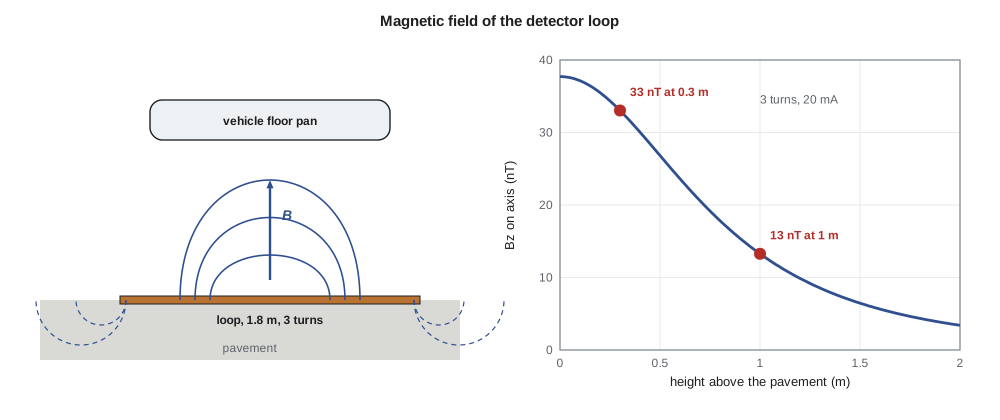
Leo pulls a typical loop from the installation drawings: a square 1.8 m on a side, three turns of insulated wire in the saw cut, driven by the detector oscillator with a current of about 20 mA. Amara computes the field by summing the Biot–Savart contributions of the four sides, numerically, at points along the axis. At the pavement surface the field is about 38 nT. It falls only slowly up to a height of about half the loop's width, reaching about 33 nT at 0.3 m, then drops faster, to about 13 nT at 1 m and 3 nT at 2 m. The car's floor pan and engine block sit in the strong, nearly uniform part of the field; a truck trailer's floor at 1.2 m sits much higher, which is why trucks with high beds are harder to detect and why loops for them are sometimes made longer or wired as quadrupoles.
Worked problem
Field at the center of the loop
Find the field at the center of the 1.8 m square loop with 3 turns carrying 20 mA, and compare it with the Earth's field.
Show solution
- \[B = \frac{2\sqrt{2}\,\mu_0 N I}{\pi s} = \frac{2\sqrt2 \times 4\pi\times10^{-7} \times 3 \times 0.020}{\pi \times 1.8}\]
- \[B = \frac{2.828 \times 7.540\times10^{-8}}{5.655} = 37.7\ \text{nT}\]
- \[\frac{B}{B_{\text{Earth}}} \approx \frac{37.7\ \text{nT}}{50\ \mu\text{T}} \approx 0.00075\]
Answer: About 38 nT, less than a thousandth of the Earth's field. The steel of a car distorts the Earth's field far more than this, but that distortion is static; the detector oscillates at tens of kilohertz and responds only to changes in its own alternating field, as lesson 5 explains.
Magnetic materials
Materials respond to magnetic fields through the magnetic moments of their electrons. Most materials are diamagnetic or paramagnetic, with relative permeability μ_r within a few parts per hundred thousand of 1; for engineering purposes they are non-magnetic. Ferromagnetic materials, such as iron, nickel, cobalt and their alloys and the ceramic ferrites, have μ_r from hundreds to many thousands because their atomic moments align in domains. In them B = μH = μ₀μ_r H, but only up to saturation, beyond which further H barely increases B. Their B–H curve also shows hysteresis: the material retains some magnetization when H returns to zero, and a cycle round the hysteresis loop dissipates energy as heat.
Ferrites are the electromagnetic engineer's everyday magnetic material. They have moderate permeability, high resistivity so that eddy currents are small, and useful behavior up to tens or hundreds of megahertz, depending on the grade. A ferrite core turns a few turns of wire into a large inductance; a ferrite sleeve over a cable adds impedance to currents flowing on the outside of the cable, which suppresses common-mode interference. On the APS-2, a snap-on ferrite on the cable to the button cap, and a ferrite bead in series with each audio line, are cheap insurance against both electrostatic discharge transients and radio-frequency pickup. Ferrite loses its permeability above its Curie temperature, so grades are chosen for the temperature range of an outdoor enclosure.
| Material | Relative permeability μ_r | Comments |
|---|---|---|
| Air, copper, aluminum, plastics, concrete | ≈ 1 | Non-magnetic for engineering purposes |
| Mild steel | hundreds to a few thousand | Saturates near 1.5–2 T; conductive, so eddy currents are large |
| Silicon steel laminations | thousands | Transformer and motor cores at power frequencies |
| Manganese-zinc ferrite | about 1000–10 000 | Power and common-mode chokes, up to a few megahertz |
| Nickel-zinc ferrite | about 20–1000 | Radio-frequency beads and cores, tens to hundreds of megahertz |
| Powdered iron | about 10–100 | Distributed air gap; stable inductors |
Magnetic boundary conditions mirror the electric ones: the normal component of B is continuous across any interface, and the tangential component of H is continuous unless a surface current flows. At the boundary between air and a high-permeability material, field lines in the air arrive almost perpendicular to the surface, just as electric field lines meet a conductor at right angles. This is how a ferrite core guides flux and how a steel plate under a loop detector, perhaps a buried steel plate from roadwork, changes the loop's inductance permanently.
Inductance
The flux Φ through a circuit, multiplied by the number of turns N that link it, is the flux linkage λ = NΦ. For a circuit in a linear medium, the flux linkage is proportional to the current that produces it, and the ratio is the self-inductance L = λ/I, in henrys. The flux linking a second circuit, divided by the current in the first, is the mutual inductance M. Inductance, like capacitance, depends only on geometry and materials. For a coaxial cable, the flux between the conductors per unit length gives L′ = (μ/2π) ln(b/a). For two parallel wires, L′ = (μ₀/π) arccosh(D/2a). A long solenoid has L = μN²A/ℓ.
For a single-turn square loop of side s made of wire of radius r, a standard approximation gives L ≈ (2μ₀s/π)[ln(s/r) − 0.774]. When N turns are bundled tightly together, the flux of each turn links all the others and the inductance grows roughly as N². The approximation ignores the internal inductance of the wire, which matters little at tens of kilohertz, and treats the bundle as a single wire with an effective radius. For a real loop in pavement, the reinforcing steel, the moisture of the ground and the sealant all shift the value slightly, so detector manufacturers quote broad ranges and the detector tunes itself to whatever it finds.
The energy stored in an inductor, ½LI², lives in its magnetic field, with density ½B·H. This view explains why inductance falls when a conducting plate approaches a loop: as lesson 5 shows, eddy currents in the plate push the field out of the space the plate occupies, reducing the total field energy for a given current, and therefore reducing L. It also explains why an inductor with a ferrite core stores most of its energy in a small air gap: the gap has a much lower permeability, so for the same B its H is much larger, and the energy density ½BH is concentrated there.
Worked problem
Inductance of the loop and lead-in
Estimate the inductance of the 3-turn, 1.8 m square loop, taking an effective bundle radius of 3 mm, and of a 50 m twisted-pair lead-in with conductors of radius 0.8 mm spaced 3.0 mm apart.
Show solution
- \[L_1 \approx \frac{2\mu_0 s}{\pi}\Big[\ln\frac{s}{r} - 0.774\Big] = \frac{2 \times 4\pi\times10^{-7} \times 1.8}{\pi}\,[\ln 600 - 0.774] = 8.10\ \mu\text{H}\]
- \[L_{\text{loop}} \approx N^2 L_1 = 9 \times 8.10 = 72.9\ \mu\text{H}\]
- \[L'_{\text{lead}} = \frac{\mu_0}{\pi}\operatorname{arccosh}\frac{3.0}{1.6} = 0.497\ \mu\text{H/m} \qquad L_{\text{lead}} = 24.8\ \mu\text{H}\]
- \[L_{\text{total}} \approx 72.9 + 24.8 = 97.7\ \mu\text{H}\]
Answer: About 98 µH, consistent with the 100 µH the ELE-340 oscillator was designed for. A quarter of it belongs to the lead-in, which adds inductance without adding sensitivity; a car changes only the loop part. That is why detectors lose sensitivity with very long lead-ins and why the lead-in must be twisted tightly, so that its own field is small and does not respond to passing vehicles.
import math
mu0 = 4e-7 * math.pi
def seg_B(p, a, b, I):
    """Biot-Savart field at p from a straight segment a -> b carrying I, summed over 400 pieces."""
    Bx = By = Bz = 0.0; n = 400
    for k in range(n):
        m = [a[i] + (b[i] - a[i]) * (k + 0.5) / n for i in range(3)]      # midpoint of the piece
        dl = [(b[i] - a[i]) / n for i in range(3)]
        R = [p[i] - m[i] for i in range(3)]; r3 = (R[0]**2 + R[1]**2 + R[2]**2) ** 1.5
        cx = dl[1]*R[2] - dl[2]*R[1]; cy = dl[2]*R[0] - dl[0]*R[2]; cz = dl[0]*R[1] - dl[1]*R[0]
        f = mu0 * I / (4 * math.pi * r3)
        Bx += f * cx; By += f * cy; Bz += f * cz
    return Bx, By, Bz
s, N, I = 1.8, 3, 0.02          # loop side 1.8 m, 3 turns, 20 mA
h = s / 2
corners = [(-h, -h, 0), (h, -h, 0), (h, h, 0), (-h, h, 0)]
def loop_Bz(p):
    return sum(seg_B(p, corners[k], corners[(k + 1) % 4], N * I)[2] for k in range(4))
print(f"origin: Biot-Savart {loop_Bz((0, 0, 0))*1e9:.1f} nT, formula {2*math.sqrt(2)*mu0*N*I/(math.pi*s)*1e9:.1f} nT")
for z in (0.15, 0.3, 0.6, 1.0, 2.0):
    print(f"height {z:4.2f} m: Bz on axis = {loop_Bz((0, 0, z))*1e9:5.1f} nT")
# inductance of the loop (square-loop approximation x N^2) and of a twisted-pair lead-in
r_eff = 0.003
L1 = 2 * mu0 * s / math.pi * (math.log(s / r_eff) - 0.774)
Dp, ap, Llead = 3.0e-3, 0.8e-3, 50.0
Lp = mu0 / math.pi * math.acosh(Dp / (2 * ap))
print(f"one turn {L1*1e6:.2f} uH, loop with {N} turns {N*N*L1*1e6:.1f} uH")
print(f"lead-in {Lp*1e6:.3f} uH/m x {Llead:.0f} m = {Lp*Llead*1e6:.1f} uH; total {(N*N*L1 + Lp*Llead)*1e6:.1f} uH")origin: Biot-Savart 37.7 nT, formula 37.7 nT height 0.15 m: Bz on axis = 36.4 nT height 0.30 m: Bz on axis = 33.0 nT height 0.60 m: Bz on axis = 23.6 nT height 1.00 m: Bz on axis = 13.3 nT height 2.00 m: Bz on axis = 3.4 nT one turn 8.10 uH, loop with 3 turns 72.9 uH lead-in 0.497 uH/m x 50 m = 24.8 uH; total 97.7 uH
The numerical Biot–Savart sum agrees with the closed-form center field, which validates the code before it is used where no formula exists, such as at points off the axis or for loops of other shapes. Amara later extends it to a diamond-shaped loop and to a long rectangular loop for a bicycle lane, where the question is whether the field over the lane edge is strong enough to detect a bicycle's small aluminum and steel parts. The inductance figures come out close to the design value of the ELE-340 oscillator; the exact value in the field will differ, and the detector's automatic tuning absorbs the difference.
Forces between currents
Two parallel wires carrying currents in the same direction attract; in opposite directions they repel. The force per meter between wires a distance d apart is μ₀I₁I₂/(2πd), which was the basis of the old definition of the ampere. At ordinary currents the force is tiny, but during a short circuit in a power distribution cabinet, tens of kiloamperes can bend busbars, so busbar supports are rated for fault forces. In the signal cabinet, the force reminds us that magnetic fields store energy and do mechanical work, the principle behind every relay that switches a lamp load and every motor that drives a gate arm.
Common mistakes
MistakeGetting the direction of B round a wire backwards.
InsteadPoint the right thumb along the current; the fingers curl in the direction of B.
MistakeUsing Ampère's law to find the field of a finite loop directly.
InsteadAmpère's law holds for any path but gives the field only with symmetry; use Biot–Savart for loops.
MistakeTreating ferrite permeability as constant.
InsteadPermeability falls with frequency and temperature and collapses at saturation; check the grade's curves.
MistakeCounting lead-in inductance as useful loop sensitivity.
InsteadA vehicle changes only the loop's inductance; a long lead-in dilutes the fractional change the detector sees.
Summary and key terms
- The magnetic force on a moving charge is qv×B; on a current element it is I dl×B.
- The Biot–Savart law gives the field of any current distribution; fields of simple shapes have closed forms.
- Ampère's law relates the circulation of H to enclosed current; ∇·B = 0 means field lines close on themselves.
- The detector loop's field is tens of nanoteslas and falls rapidly above about half the loop width.
- Ferromagnetic materials and ferrites raise μ_r greatly but saturate, show hysteresis and vary with frequency.
- Inductance is flux linkage per ampere; it depends on geometry and materials and stores energy ½LI² in the field.
- Magnetic flux density
- B, in teslas, defined by the force on a moving charge.
- Magnetic field intensity
- H = B/μ, in amperes per meter.
- Biot–Savart law
- The law giving the magnetic field produced by a current element.
- Ampère's circuital law
- The circulation of H round a closed path equals the current enclosed.
- Permeability
- μ = μ₀μ_r, the ratio of B to H in a material.
- Hysteresis
- Dependence of a ferromagnet's magnetization on its history, causing loss each cycle.
- Self-inductance
- Flux linkage of a circuit per unit of its own current.
- Mutual inductance
- Flux linkage of one circuit per unit current in another.
Practice problems
Work each problem on paper first, then reveal the answer to check.
Find the field 5 cm from a long wire carrying 10 A.
Show answer
μ₀I/(2πρ) = 40 µT.
Find the field at the center of a circular loop of radius 0.5 m with 4 turns carrying 50 mA.
Show answer
μ₀NI/(2a) = 0.251 µT.
A coaxial cable has a = 0.45 mm and b = 1.475 mm with a non-magnetic dielectric. Find L′.
Show answer
(μ₀/2π) ln(3.278) = 0.237 µH/m.
A solenoid has 200 turns on a 2 cm diameter former 5 cm long. Estimate its inductance.
Show answer
μ₀N²A/ℓ = 4π × 10⁻⁷ × 40 000 × 3.14 × 10⁻⁴ / 0.05 = 316 µH.
Two wires 2 cm apart each carry 100 A in opposite directions. Find the force per meter.
Show answer
μ₀I²/(2πd) = 0.1 N/m, repulsive.
How much energy does a 100 µH loop store at 20 mA?
Show answer
½LI² = 20 nJ.
Lesson quiz · 5 questions
Score 60% or more to complete this lesson.
Create a free account to save your progress, take quizzes and earn a certificate.