
ELE-360 · Lesson 3 of 12 · 24 min
Conductors, dielectrics and capacitance
Lesson 2 treated charges in empty space. Real products are made of materials, and materials change fields. Metals let charge flow freely, so they shape fields by rearranging their surface charge. Insulators do not conduct, but their molecules polarize, reducing the field for a given charge and storing more energy. Where two materials meet, the fields obey boundary conditions that decide how field lines bend, where charge collects and how much capacitance a structure has. This lesson develops those ideas and applies them to three things on Amara's bench: the coaxial cable that feeds the TLR-1 antenna, the printed-circuit trace that carries the radio signal across the board, and the button cap whose capacitance to the enclosure decides how an electrostatic discharge divides its current.
Conductors and current density
In a conductor, some electrons are free to move. An applied field E drives them, and the resulting current density J, in amperes per square meter, is proportional to the field: J = σE, where σ is the conductivity in siemens per meter. This is Ohm's law at a point. Integrating over a uniform wire of length ℓ and cross-section A recovers the familiar R = ℓ/(σA). Copper has σ ≈ 5.8 × 10⁷ S/m, aluminum about 3.5 × 10⁷ S/m and stainless steel roughly 1.4 × 10⁶ S/m, while seawater manages about 4 S/m and wet soil anywhere from 10⁻³ to 10⁻¹ S/m. The range spans more than twenty orders of magnitude from good conductors to good insulators, which is why a single symbol σ, and later a single loss parameter, can describe everything from a copper trace to a concrete pole footing.
Charge placed inside a conductor does not stay there. Combining J = σE with Gauss's law and the continuity equation, ∇·J = −∂ρ_v/∂t, shows that any interior charge density decays exponentially with a relaxation time τ = ε/σ. For copper τ is about 10⁻¹⁹ s, effectively instantaneous; the charge rushes to the surface. For a poor conductor such as dry concrete τ can be milliseconds or longer, which is why charge can linger on a dry pole or a plastic bezel. The relaxation time gives a useful test: a material behaves as a conductor at frequencies well below 1/(2πτ) and as a dielectric well above it.
Dielectrics and polarization
An insulator, or dielectric, has no free charge, but an applied field stretches its atoms and rotates its polar molecules, producing tiny dipoles. The dipole moment per unit volume is the polarization P. The bound charges at the ends of the dipoles partly cancel the applied field inside the material. Rather than track bound charge, we absorb it into the electric flux density: D = ε₀E + P = εE, where ε = ε₀ε_r and ε_r is the relative permittivity or dielectric constant. Gauss's law in the form ∮D·dS = Q_free then holds in any linear material, counting only the free charge. A capacitor filled with a dielectric of ε_r holds ε_r times as much charge at the same voltage.
| Material | Typical ε_r | Typical dielectric strength | Where it appears |
|---|---|---|---|
| Air | 1.0006 | about 3 MV/m | Everywhere |
| PTFE | 2.1 | tens of MV/m | Low-loss coaxial cable, RF boards |
| Polyethylene (solid) | 2.25 | tens of MV/m | Coaxial cable dielectric |
| Polycarbonate | about 2.9 | about 15 MV/m | APS-2 bezel and radome |
| FR-4 glass-epoxy | about 4.2–4.7 near 1 GHz | about 20 MV/m | Printed-circuit boards |
| Glass | about 5–7 | varies widely | Windows, cabinet viewing ports |
| Concrete | about 4–10, rising with moisture | varies widely | Poles, pavement, buildings |
| Water | about 80 at low frequency | varies | Rain, wet ground, ice-free puddles |
Real dielectrics are not perfect. Their polarization lags the field a little at high frequency, which turns some field energy into heat. We describe this with a complex permittivity ε = ε′ − jε″, or with the loss tangent tan δ = ε″/ε′. FR-4 has a loss tangent of roughly 0.02 near 1 GHz, PTFE about 0.0002. At 915 MHz this difference is noticeable on a long trace but not dramatic; at tens of gigahertz it decides the choice of board material. Every dielectric also has a dielectric strength, the field at which it breaks down. The table gives typical values; thin films and good insulators are much stronger than air, which is why insulating spacers and conformal coatings raise the voltage a circuit can withstand.
Boundary conditions
At the interface between two materials, the field changes abruptly, but in a controlled way. Applying Faraday's law round a thin rectangle straddling the boundary shows that the tangential component of E is continuous: E_t1 = E_t2. Applying Gauss's law to a thin pillbox shows that the normal component of D jumps by any free surface charge: D_n1 − D_n2 = ρ_S. At a boundary between two dielectrics with no free charge, the normal D is continuous, so the normal E is larger in the material with the smaller permittivity. Field lines therefore bend at the interface, and the ratio of the tangents of the angles they make with the normal equals the ratio of the permittivities.
At a conductor surface, with the conductor as medium 2, the field inside is zero. So the tangential field just outside is zero too, and the normal D equals the surface charge density. These two rules, E tangential = 0 and D normal = ρ_S, are the conductor boundary conditions you will use in every later lesson, including the waveguides of lesson 11, where the requirement of zero tangential field on the metal walls determines which waves can propagate. They also explain a practical effect: an air gap in series with a dielectric carries a stronger field than the dielectric, so a thin layer of air trapped under a conformal coating or in a void in an insulator can break down first, producing partial discharge.
Capacitance
Two conductors carrying equal and opposite charges ±Q with a potential difference V between them form a capacitor of capacitance C = Q/V. Capacitance depends only on the geometry and the materials, not on the charge. To find it, assume a charge, find the field from Gauss's law or by solving Laplace's equation, integrate the field to find V and divide. For parallel plates of area A and spacing d filled with ε, the field is uniform and C = εA/d, ignoring the fringing field at the edges. For a coaxial cable with inner radius a and outer radius b, Gauss's law on a cylinder between them gives the field ρ_L/(2περ), and integrating from a to b gives the capacitance per unit length. For two parallel wires and for a wire over a ground plane, the method of images gives closed forms too.
| Structure | Capacitance | Notes |
|---|---|---|
| Parallel plates, area A, spacing d | C = εA/d | Neglects fringing; good when d is small compared with the plate size |
| Coaxial cable, radii a and b | C′ = 2πε/ln(b/a) per meter | Exact for a uniform cable |
| Isolated sphere, radius a | C = 4πε₀a | About 111 pF for a = 1 m |
| Wire of radius a, height h over ground | C′ = 2πε₀/arccosh(h/a) per meter | Method of images |
| Two parallel wires, radius a, spacing D | C′ = πε₀/arccosh(D/2a) per meter | Twin-lead, twisted pair approximately |
The method of images deserves a sentence of its own because it appears again and again. A charge above a flat, grounded conducting plane produces exactly the same field above the plane as the charge together with an equal and opposite image charge the same distance below, with the plane removed. The image arrangement satisfies the same boundary condition, V = 0 on the plane, and by uniqueness it must give the right answer. A wire over a ground plane becomes a pair of wires; a monopole antenna over a ground plane becomes a dipole, which is why lesson 12 can analyze the TLR-1 whip as half of a dipole.
Worked problem
Capacitance of the antenna feeder
The TLR-1 cabinet antenna is fed through a coaxial cable with a center conductor of radius 0.45 mm and a solid polyethylene dielectric (ε_r = 2.25) of outer radius 1.475 mm, similar to the common 50 Ω flexible cable. Find the capacitance per meter and the capacitance of a 12 m run.
Show solution
- \[C' = \frac{2\pi\varepsilon_0\varepsilon_r}{\ln(b/a)} = \frac{2\pi \times 8.854\times10^{-12} \times 2.25}{\ln(1.475/0.45)}\]
- \[\ln(3.278) = 1.187 \qquad C' = \frac{1.252\times10^{-10}}{1.187} = 105.4\ \text{pF/m}\]
- \[C = 12 \times 105.43\ \text{pF} = 1.27\ \text{nF}\]
Answer: About 105 pF/m, close to the 100 pF/m or so that datasheets list for this class of cable, and 1.27 nF for the run. At 915 MHz this capacitance is not a lumped load; it is distributed along the line with its inductance, and lesson 9 shows how the two together give the cable its characteristic impedance.
Solving Laplace's equation numerically
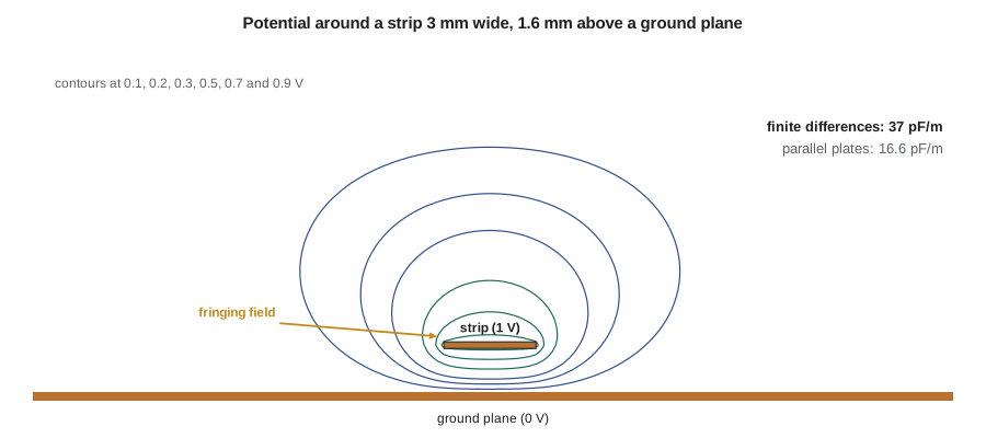
Most real structures lack the symmetry that makes Gauss's law easy. A printed-circuit trace above a ground plane, for example, has a strong field under the trace and a fringing field that curls out from its edges into the air. To find its capacitance, Amara solves Laplace's equation on a grid. The finite-difference form of ∇²V = 0 in two dimensions says that each grid potential is the average of its four neighbors. Set the trace to 1 V and the ground plane and enclosure walls to 0 V, sweep the grid repeatedly replacing each free value by the average of its neighbors, and the values converge to the solution. Successive over-relaxation, which overshoots each update by a factor ω between 1 and 2, speeds convergence greatly. The charge on the trace follows from Gauss's law applied round a rectangle enclosing it, and C′ = Q′/V.
import math
eps0 = 8.854e-12
# 1. Coaxial feeder (50 ohm class, solid polyethylene)
a, b, er = 0.45e-3, 1.475e-3, 2.25
Cc = 2 * math.pi * eps0 * er / math.log(b / a)
print(f"coax: C' = {Cc*1e12:.1f} pF/m, 12 m run = {12*Cc*1e9:.2f} nF")
# 2. Relaxation time tau = eps / sigma for some materials
for name, er_, sig in (("copper", 1, 5.8e7), ("seawater", 81, 4.0), ("wet soil", 15, 1e-2), ("dry concrete", 5, 1e-6)):
    tau = er_ * eps0 / sig
    print(f"{name:12s} tau = {tau:.2e} s, conductor-like below about {1/(2*math.pi*tau):.2e} Hz")
# 3. Finite-difference Laplace solution: strip 3.0 mm wide, 1.6 mm above ground, in air
d = 0.1e-3                              # grid step 0.1 mm
NX, NY = 300, 100                       # box 30 mm wide, 10 mm tall, walls at 0 V
jy, i0, i1 = 16, 135, 165               # strip row and columns
V = [ [0.0] * NX for _ in range(NY) ]
fixed = [ [j in (0, NY - 1) or i in (0, NX - 1) for i in range(NX)] for j in range(NY) ]
for i in range(i0, i1 + 1): V[jy][i] = 1.0; fixed[jy][i] = True
w = 1.95                                # over-relaxation factor
for it in range(600):
    for j in range(1, NY - 1):
        Vj, Vu, Vd, fj = V[j], V[j + 1], V[j - 1], fixed[j]
        for i in range(1, NX - 1):
            if not fj[i]:
                Vj[i] += w * (0.25 * (Vj[i - 1] + Vj[i + 1] + Vu[i] + Vd[i]) - Vj[i])
# charge per unit length from Gauss's law round a rectangle enclosing the strip
jl, jh, il, ih = jy - 8, jy + 8, i0 - 8, i1 + 8
Q = 0.0
for i in range(il, ih):
    Q += eps0 * ((V[jh][i] - V[jh + 1][i]) + (V[jl][i] - V[jl - 1][i]))
for j in range(jl, jh):
    Q += eps0 * ((V[j][il] - V[j][il - 1]) + (V[j][ih] - V[j][ih + 1]))
wh = 3.0 / 1.6
Z0air = 120 * math.pi / (wh + 1.393 + 0.667 * math.log(wh + 1.444))   # closed-form fit, used in lesson 11
print(f"strip over ground: C' = {Q*1e12:.1f} pF/m by finite differences")
print(f"parallel-plate estimate eps0*w/h = {eps0*wh*1e12:.1f} pF/m; closed-form fit 1/(c Z0) = {1/(2.998e8*Z0air)*1e12:.1f} pF/m")coax: C' = 105.4 pF/m, 12 m run = 1.27 nF copper tau = 1.53e-19 s, conductor-like below about 1.04e+18 Hz seawater tau = 1.79e-10 s, conductor-like below about 8.88e+08 Hz wet soil tau = 1.33e-08 s, conductor-like below about 1.20e+07 Hz dry concrete tau = 4.43e-05 s, conductor-like below about 3.60e+03 Hz strip over ground: C' = 37.0 pF/m by finite differences parallel-plate estimate eps0*w/h = 16.6 pF/m; closed-form fit 1/(c Z0) = 36.0 pF/m
The coaxial result matches the worked example. The relaxation times show why copper behaves as a conductor at any frequency of interest, while seawater is a conductor up to the high megahertz and dry concrete acts mostly as a dielectric above a few kilohertz; the numbers depend strongly on moisture, so treat them as orders of magnitude. The finite-difference solution gives about 37 pF/m for the strip, more than twice the parallel-plate estimate of 16.6 pF/m, because the fringing field round the edges and over the top carries as much charge as the field directly underneath. A closed-form curve fit for microstrip, which lesson 11 uses to design traces, gives about 36 pF/m; the small difference comes from the enclosure walls in the numerical model and the finite grid. On a real board the field below the trace lies in FR-4 and the field above it in air, so the trace sees an effective permittivity between 1 and 4.4, a point lesson 11 develops.
Energy and force in capacitors
A capacitor charged to V stores W = ½CV² = ½QV = Q²/(2C). The energy is in the field, with density ½εE², so a dielectric with a high ε_r stores more energy in the same field. The stored energy also produces forces: the plates of a charged capacitor attract each other with a force equal to the rate of change of energy with spacing at constant charge. These forces are small at ordinary voltages but are the operating principle of electrostatic actuators and of the microelectromechanical accelerometers in many modern devices. In the APS-2 they matter in a different way: high-permittivity ceramic capacitors change capacitance with applied voltage and temperature, which shifted the resonant frequency of an early loop-detector oscillator until Amara changed to a stable dielectric type.
The button cap as a capacitor
Back to electrostatic discharge. The button cap and the station's metal enclosure form a capacitor through the plastic bezel; so do the cap and the button-sense trace on the board beneath it. When a charged finger arcs to the cap, the discharge current divides among the paths from the cap to ground in proportion to their admittance at the very high frequencies in the pulse. A short bond strap from the cap to the enclosure has low inductance and wins; without it, the capacitance from the cap to the sense trace, a few picofarads, carries a large share of a current that rises at tens of amperes per nanosecond. Amara's numbers suggest the first pilot's damage came from exactly this path. Her change list for the next build includes a bonding spring from the cap to the enclosure, a guard ring of grounded copper round the sense pad and a series resistor with a clamp at the input.
Common mistakes
MistakeUsing D = εE across a boundary for the tangential component.
InsteadTangential E is continuous; normal D is continuous only when there is no free surface charge.
MistakeUsing C = εA/d for a narrow trace over ground.
InsteadFringing fields roughly double the capacitance of a trace whose width is similar to its height; solve numerically or use a fitted formula.
MistakeAssuming a dielectric's ε_r is a fixed number.
InsteadPermittivity varies with frequency, temperature, moisture and, for high-ε ceramics, applied voltage.
MistakeForgetting the image charge has the opposite sign.
InsteadThe image of a charge in a grounded plane is equal and opposite and mirrored below the plane.
Summary and key terms
- Conductors obey J = σE; interior charge relaxes to the surface in τ = ε/σ.
- Dielectrics polarize; D = εE with ε = ε₀ε_r, and Gauss's law counts only free charge.
- Complex permittivity and the loss tangent describe dielectric loss; every insulator has a breakdown strength.
- Tangential E is continuous at a boundary; normal D jumps by the free surface charge; at a conductor E_t = 0 and D_n = ρ_S.
- Capacitance depends on geometry and materials; coax, parallel plates and image methods have closed forms.
- Laplace's equation solved on a grid gives capacitance of structures without symmetry, including fringing.
- Conductivity
- σ, the ratio of current density to electric field in a conductor, in S/m.
- Relaxation time
- τ = ε/σ, the time constant for interior charge in a material to decay.
- Polarization
- Dipole moment per unit volume induced in a dielectric by an applied field.
- Relative permittivity
- ε_r, the factor by which a material increases the flux density for a given field.
- Loss tangent
- tan δ = ε″/ε′, a measure of energy lost in a dielectric per cycle.
- Boundary conditions
- Rules relating fields on the two sides of an interface between materials.
- Method of images
- Replacing a conducting plane by image charges that reproduce its boundary condition.
- Fringing field
- The part of a capacitor's field that spreads beyond the region between its conductors.
Practice problems
Work each problem on paper first, then reveal the answer to check.
A 30 m copper conductor has a 1.5 mm² cross-section. What is its resistance?
Show answer
30 / (5.8 × 10⁷ × 1.5 × 10⁻⁶) = 0.345 Ω.
Find the capacitance of plates 20 mm × 20 mm, 0.2 mm apart, filled with FR-4 of ε_r = 4.4, ignoring fringing.
Show answer
εA/d = 4.4 × 8.854 × 10⁻¹² × 4 × 10⁻⁴ / 2 × 10⁻⁴ = 77.9 pF.
A field of 2 kV/m in air meets a polycarbonate sheet (ε_r = 2.9) normally. What is the field inside the sheet?
Show answer
Normal D is continuous, so E = 2/2.9 = 0.69 kV/m.
A wire of radius 1 mm runs 10 mm above a ground plane. Find its capacitance per meter.
Show answer
2πε₀/arccosh(10) = 55.6 × 10⁻¹² / 2.993 = 18.6 pF/m.
What is the relaxation time of seawater (ε_r = 81, σ = 4 S/m)?
Show answer
81 × 8.854 × 10⁻¹² / 4 = 1.79 × 10⁻¹⁰ s.
A 100 pF capacitor is charged to 500 V. How much energy does it store?
Show answer
½CV² = 12.5 µJ.
Lesson quiz · 5 questions
Score 60% or more to complete this lesson.
Create a free account to save your progress, take quizzes and earn a certificate.