
ELE-360 · Lesson 12 of 12 · 26 min
Antennas and the TLR-1 antenna design
An antenna is the structure that turns a guided wave on a transmission line into a wave traveling through space, and back again. Every idea in this course meets in it. Its currents follow Maxwell's equations; its fields near the structure are the quasi-static electric and magnetic fields of lessons 2 to 5; its far fields are plane waves carrying power by the Poynting vector; it must be matched to its feeder; and its performance depends on the metal and dielectric around it. This final lesson explains how antennas radiate, introduces the short dipole, the half-wave dipole and the monopole, defines the quantities on an antenna datasheet, connects them through the Friis transmission equation, and then follows Amara through the antenna and feeder design of the TLR-1 pole station and cabinet, with the electromagnetic-compatibility and exposure checks that go with it.
How antennas radiate
A static charge has a static field and a steady current a static magnetic field; neither radiates. Radiation needs accelerating charge, that is, a time-varying current. Picture the electric field lines between the two arms of a short dipole driven by a sinusoidal source. As the charge on the arms reverses each half cycle, the field lines near the antenna must reverse too, but the field farther out cannot respond instantly: changes travel outward at the speed of light. The field lines stretch, pinch off and form closed loops that keep moving outward, sustained by the changing magnetic field they create, exactly the self-sustaining wave predicted by Maxwell. Once the loops are more than about a wavelength away, they form an expanding spherical wave that is locally a plane wave.
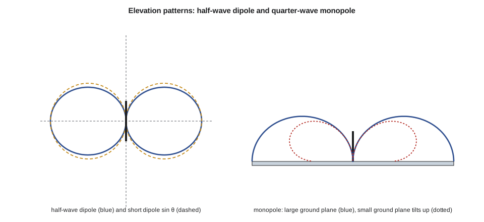
Mathematically, the retarded vector potential of lesson 6 gives the fields of a short current element I dl directly. Close to the element, within about λ/2π, the fields are dominated by terms falling as 1/r³ and 1/r², the reactive near field, which stores energy and returns it each cycle like the field of a capacitor or inductor. Far from the element, the terms falling as 1/r dominate: E_θ and H_φ, perpendicular to each other and to the radial direction, in the ratio η₀, carrying power outward. The far field of a short dipole along z is proportional to sin θ: maximum broadside, zero along the axis. This is the antenna's radiation pattern.
Radiation resistance, directivity and gain
Integrating the Poynting vector over a sphere gives the total radiated power, and dividing by ½I² defines the radiation resistance R_rad: the resistance that would dissipate the radiated power if the antenna were a resistor. For a short dipole with uniform current, the Hertzian dipole, R_rad = 80π²(dl/λ)²; a real short dipole has current falling to zero at its tips, roughly triangular, and a quarter of that value. Short antennas therefore have tiny radiation resistances. Any loss resistance in the conductors, the matching network or the ground competes with R_rad, and the radiation efficiency η_rad = R_rad/(R_rad + R_loss) can be poor. A 2 cm monopole at 915 MHz has a radiation resistance of about 1.5 Ω; with 1 Ω of loss it is only about 60 percent efficient, and it is also very narrowband.
Directivity D is the ratio of the radiation intensity in the strongest direction to the average over all directions; an isotropic antenna, radiating equally everywhere, would have D = 1. The short dipole has D = 1.5, or 1.76 dBi, the 'i' meaning relative to isotropic. Gain G = η_rad D includes losses, and realized gain also includes mismatch loss. Antenna datasheets quote gain in dBi, or in dBd relative to a half-wave dipole, which is 2.15 dB above isotropic. The product of transmitter power and antenna gain, less feeder loss, is the effective isotropic radiated power, EIRP, which regulators limit.
The half-wave dipole and the monopole
The half-wave dipole, two quarter-wave arms fed at the center, is the reference antenna of radio engineering. Its current is close to a half sinusoid along its length, maximum at the feed and zero at the tips. Integrating the fields of that current distribution gives a pattern slightly narrower than sin θ, a directivity of 1.64 (2.15 dBi) and a radiation resistance of about 73 Ω, with a small inductive reactance that disappears when the dipole is shortened by a few percent. The input impedance near 73 Ω matches 75 Ω coaxial cable well and 50 Ω cable acceptably; real dipoles are trimmed and matched to 50 Ω.
A monopole is one arm of a dipole standing on a ground plane. By the method of images of lesson 3, the ground plane supplies the missing half, so above the plane the fields are those of a dipole. The monopole radiates only into the half-space, so its radiation resistance is half the dipole's, about 36.5 Ω for a quarter-wave monopole, and its directivity is double, about 5.15 dBi on an infinite plane. On a real, finite ground plane such as a small metal enclosure or a mast arm, the pattern tilts upward, the gain falls toward that of a dipole and some current flows on the outside of the feeder, which then radiates too. The quarter-wave whip at 915 MHz is about 82 mm long, trimmed a few percent shorter to allow for the thickness of the element and the end effect.
| Antenna | Radiation resistance | Directivity | Notes |
|---|---|---|---|
| Short (Hertzian) dipole, uniform current | 80π²(dl/λ)² | 1.5 (1.76 dBi) | Theoretical building block |
| Short dipole, triangular current | 20π²(l/λ)² | 1.5 (1.76 dBi) | Realistic short antenna |
| Half-wave dipole | about 73 Ω | 1.64 (2.15 dBi) | Reference antenna |
| Quarter-wave monopole, large ground | about 36.5 Ω | 3.28 (5.15 dBi) | Whip on a vehicle roof or enclosure |
| Small loop, area A | 320π⁴(A/λ²)² per turn² | 1.5 (1.76 dBi) | Magnetic dipole; very low R_rad |
| Patch or panel antenna | matched to 50 Ω | about 6–9 dBi | Directional; used on the cabinet mast arm |
Effective aperture and the Friis equation
A receiving antenna collects power from an incident wave as if it presented an area to it. This effective aperture A_e is related to gain by A_e = λ²G/(4π), a consequence of reciprocity: an antenna's receiving and transmitting properties are identical. A 2 dBi antenna at 915 MHz has an effective aperture of about 135 cm², a 6 dBi panel about 340 cm². Combining the power density of a transmitting antenna at distance d, P_tG_t/(4πd²), with the effective aperture of the receiving antenna gives the Friis transmission equation, which ELE-350 used for link budgets. In decibels, the received power equals the transmitted power plus both gains minus the free-space path loss 20 log(4πd/λ). Lesson 7's plane-wave power density and this lesson's aperture are the field-theory content behind that simple sum.
The Friis equation holds in the far field of both antennas, beyond about 2D²/λ for an antenna of largest dimension D, and beyond a few wavelengths for small antennas. Inside the reactive near field, within about λ/2π (5.2 cm at 915 MHz), the antenna is strongly coupled to anything nearby: a hand, a metal enclosure or another antenna changes its impedance and pattern. That is the electromagnetic reason a radio's antenna must not be mounted flat against metal, and why the antenna specification for the pole station requires a clearance of at least a few centimeters from the enclosure walls in every direction except the ground plane beneath it.
Design: the pole station antenna
The TLR-1 pole station lives in the APS-2 push-button housing on the pedestrian pole, a cast aluminum box. Lesson 8 showed that the box is effectively opaque at 915 MHz, so the antenna must be outside it or behind a window. Amara compares three options. A printed inverted-F antenna inside the box behind a plastic window is cheap but would sit within the reactive near field of the metal walls, with poor efficiency and a pattern set by the window. A short helical whip on top of the box is compact but, like any antenna much smaller than a quarter wavelength, has low radiation resistance and narrow bandwidth. A quarter-wave monopole on the top face, which acts as its ground plane, under the 3 mm polycarbonate cap of lesson 8, is 78 mm tall, efficient and broad enough for 902–928 MHz.
She chooses the quarter-wave monopole. Its ground plane, the top of the 120 × 160 mm housing, is less than half a wavelength across, so the pattern tilts upward and the gain toward the horizon is about 2 dBi rather than the 5 dBi of an infinite plane, the figure the ELE-350 link budget assumed. The cap costs about 0.01 dB. The pole itself, a few centimeters behind the antenna, shadows a sector of the pattern by a few decibels, so the installation instructions orient the housing with the antenna on the side facing the intersection. The antenna's feed is a short 50 Ω microstrip from the radio module and a bulkhead connector, with the coaxial shield bonded all round to the housing at the entry, following lesson 11, so that no common-mode current flows on cables leaving the box.
Worked problem
Checking the pole link with the Friis equation
A pole station transmits 14 dBm into a 2 dBi antenna, the receiving pole station's antenna is also 2 dBi, the total cable and connector loss is 2 dB and the path is 45 m. Find the free-space path loss and the received power, and compare with the ELE-350 budget, which included 15 dB of shadowing for a bus.
Show solution
- \[\lambda = 0.3277\ \text{m} \qquad L_{\text{fs}} = 20\log_{10}\frac{4\pi \times 45}{0.3277} = 64.7\ \text{dB}\]
- \[P_r = 14 + 2 + 2 - 2 - 64.7 = -48.7\ \text{dBm}\]
- \[P_r - 15\ \text{dB} = -63.7\ \text{dBm}\]
Answer: −48.7 dBm in free space and −63.7 dBm with the bus allowance, matching the ELE-350 figure, with about 40 dB of margin over the −105 dBm sensitivity. The electromagnetic design of this lesson confirms the gains that budget assumed.
Design: the cabinet antenna and feeder
The cabinet-to-cabinet link, 600 m along the arterial road, uses a 6 dBi vertically polarized panel on the mast arm at 6 m, fed by the 12 m low-loss cable chosen in lesson 9, with about 1.7 dB of cable and connector loss. The panel's measured impedance of 70 + j15 Ω is matched to better than VSWR 1.2 by the small L-network fitted by the supplier, following lesson 10. Its far field begins about 0.55 m away, so the mast arm, 0.4 m behind it, lies in its near field; the mounting bracket holds it 0.25 m off the arm with a non-conducting standoff, and Leo's measurements show the pattern and match are unchanged with the panel on the arm. A coaxial lightning arrester at the cabinet entry, bonded to the cabinet's ground bar with a short, wide strap, diverts surge currents from a nearby strike to ground before they reach the radio, and its small insertion loss is included in the 1.7 dB.
import math
c = 2.998e8; f = 915e6; lam = c / f
print(f"wavelength {lam * 1000:.1f} mm; quarter wave {lam / 4 * 1000:.1f} mm")
# 1. Short monopoles (half of a short dipole with triangular current) versus the quarter-wave whip
for L in (0.02, 0.04):
    Rr = 20 * math.pi ** 2 * (2 * L / lam) ** 2 / 2
    print(f"monopole {L * 1000:4.0f} mm: radiation resistance {Rr:5.2f} ohm, efficiency with 1 ohm loss {Rr / (Rr + 1) * 100:5.1f} %")
print(f"quarter-wave monopole: about 36.5 ohm, efficiency with 1 ohm loss {36.5 / 37.5 * 100:5.1f} %")
# 2. Half-wave dipole: radiation resistance and directivity by numerical integration of its pattern
N = 20000; I = 0.0
for k in range(N):
    th = (k + 0.5) * math.pi / N
    I += math.cos(math.pi / 2 * math.cos(th)) ** 2 / math.sin(th) * math.pi / N
D = 2 / I
print(f"half-wave dipole: Rrad = {60 * I:.1f} ohm, directivity {D:.3f} = {10 * math.log10(D):.2f} dBi")
print(f"Hertzian dipole: {10 * math.log10(1.5):.2f} dBi; quarter-wave monopole on a very large plane: {10 * math.log10(2 * D):.2f} dBi")
# 3. Friis check of the pole link, and the cabinet link in free space
def fspl(d): return 20 * math.log10(4 * math.pi * d / lam)
Pr = 14 + 2 + 2 - 2 - fspl(45)
print(f"pole link 45 m: path loss {fspl(45):.1f} dB, received {Pr:.1f} dBm free space, {Pr - 15:.1f} dBm with a bus")
Pc = 20 + 6 + 6 - 2 * 1.7 - fspl(600)
print(f"cabinet link 600 m: free-space path loss {fspl(600):.1f} dB, received {Pc:.1f} dBm before ground-reflection and shadowing losses")
# 4. Effective aperture and field regions
for G in (2, 6):
    print(f"G = {G} dBi: effective aperture {lam ** 2 * 10 ** (G / 10) / (4 * math.pi) * 1e4:.0f} cm^2")
print(f"reactive near field within about {lam / (2 * math.pi) * 100:.1f} cm; far field of a 0.30 m panel beyond {2 * 0.30 ** 2 / lam:.2f} m")
# 5. Polarization loss if a pole station is mounted tilted
for tilt in (10, 20, 30):
print(f"tilted {tilt} deg from vertical: polarization loss {-10 * math.log10(math.cos(math.radians(tilt)) ** 2):.2f} dB")wavelength 327.7 mm; quarter wave 81.9 mm monopole 20 mm: radiation resistance 1.47 ohm, efficiency with 1 ohm loss 59.5 % monopole 40 mm: radiation resistance 5.88 ohm, efficiency with 1 ohm loss 85.5 % quarter-wave monopole: about 36.5 ohm, efficiency with 1 ohm loss 97.3 % half-wave dipole: Rrad = 73.1 ohm, directivity 1.641 = 2.15 dBi Hertzian dipole: 1.76 dBi; quarter-wave monopole on a very large plane: 5.16 dBi pole link 45 m: path loss 64.7 dB, received -48.7 dBm free space, -63.7 dBm with a bus cabinet link 600 m: free-space path loss 87.2 dB, received -58.6 dBm before ground-reflection and shadowing losses G = 2 dBi: effective aperture 135 cm^2 G = 6 dBi: effective aperture 340 cm^2 reactive near field within about 5.2 cm; far field of a 0.30 m panel beyond 0.55 m tilted 10 deg from vertical: polarization loss 0.13 dB tilted 20 deg from vertical: polarization loss 0.54 dB tilted 30 deg from vertical: polarization loss 1.25 dB
The first lines show why short antennas disappoint: a 2 cm monopole has a radiation resistance of about 1.5 Ω and loses 40 percent of its power in a single ohm of loss, while the quarter-wave whip loses under 3 percent. The integration recovers the half-wave dipole's 73.1 Ω and 2.15 dBi from its current distribution, and doubling for a monopole on a large plane gives 5.16 dBi. The pole link reproduces the ELE-350 numbers. The cabinet link's free-space figure of about −59 dBm is a starting point; the ground reflection of lesson 8 and the Fresnel-zone and shadowing allowances in ELE-350's budget bring it down to the margins found there. The tilt figures support a simple installation rule: keep pole stations within about 10° of vertical, which costs less than 0.2 dB.
Electromagnetic compatibility and compliance
An antenna radiates whatever it is fed, so the TLR-1's output filter must suppress harmonics at 1830 MHz, 2745 MHz and above to the levels the spectrum rules require, and the enclosure, cables and grounding of lessons 8 and 11 must keep the digital circuits' noise from leaking out by other paths. Coexistence inside the cabinet matters too. The loop detector's 71 kHz fields and their harmonics are far below 915 MHz and do not interfere directly, but a detector's switching power supply can produce broadband noise that reaches the radio through shared wiring, so Amara puts the radio on its own filtered supply. Other radios in the cabinet, cellular modems at 700–900 MHz and Wi-Fi at 2.4 GHz, are kept apart by antenna placement and by the radio's band filter.
For the United States, the TLR-1 needs FCC equipment authorization as an intentional radiator under Part 15, section 15.247 for the 902–928 MHz band, with the radio-frequency exposure evaluation of Part 1 against the limits of section 1.1310, which lesson 7's numbers show are met with a large margin at the distances involved; the APS-2's digital circuits are unintentional radiators under Part 15. The electrostatic discharge and immunity tests of lesson 2 are part of the customer's product specification. Amara books pre-compliance scans at a test laboratory before the formal tests, so that any harmonic, enclosure or cable problem is found while it is still cheap to fix.
Design review
Amara's design review summarizes the electromagnetic decisions of the whole course. The button cap is bonded to the housing with a short spring, the sense input has a guard ring, series resistor and clamp, and sensitive traces are routed over a continuous plane, well away from the discharge path (lessons 2, 3 and 5). The redesigned detector uses tightly twisted lead-ins, staggered frequencies and a frequency-and-loss measurement to distinguish vehicles from pavement drift (lessons 4 and 5). The radio's board is a four-layer stack-up with 0.38 mm 50 Ω microstrip, a continuous ground plane, stitching vias and a shield can, and the codec clock has a 33 Ω series termination (lessons 9 and 11). The enclosure's lid seam is closed with fasteners at under 16 mm spacing and lined with absorber against cavity resonances (lessons 8 and 11). The pole antenna is a quarter-wave monopole under a thin cap, and the cabinet uses a matched 6 dBi panel on a standoff with a low-loss feeder, a weatherproofed connector and a bonded lightning arrester (lessons 8, 9, 10 and 12).
Daniel signs the review with one action item, the same kind ELE-350 ended with: measure the pole station's pattern on a real pole, with a real person pressing the button, because a hand on the housing is within the antenna's near field. Leo schedules it for the next field visit. That is how electromagnetics is practiced in a product company: models and calculations to choose the design, measurements to confirm it, and a habit of asking where the fields actually are.
Common mistakes
MistakeChoosing a very short antenna to save space without checking efficiency.
InsteadR_rad falls as the square of length; small antennas need very low loss and are narrowband.
MistakeQuoting monopole gain for an infinite ground plane.
InsteadA small ground plane tilts the beam upward and reduces gain at the horizon toward that of a dipole.
MistakeApplying the Friis equation in the near field.
InsteadUse it beyond about 2D²/λ and a few wavelengths; closer, antennas couple reactively.
MistakeMounting an antenna flat against metal or inside a metal box.
InsteadKeep the reactive near field, about λ/2π, clear of metal except the intended ground plane.
Summary and key terms
- Radiation requires time-varying current; near fields store energy and far fields carry it away as spherical waves.
- Radiation resistance, directivity, efficiency and gain describe an antenna; short antennas have tiny R_rad.
- The half-wave dipole has about 73 Ω and 2.15 dBi; a quarter-wave monopole on a large plane has about 36.5 Ω and 5.15 dBi.
- Effective aperture A_e = λ²G/(4π) and the Friis equation give received power in the far field.
- Ground plane size, nearby metal and orientation change real antenna performance; match and polarization matter too.
- The TLR-1 design combines matched antennas, low-loss feeders, shielding, grounding and compliance checks drawn from the whole course.
- Radiation pattern
- The variation of an antenna's radiated field or power with direction.
- Radiation resistance
- The resistance that would dissipate the power an antenna radiates.
- Directivity
- The ratio of peak radiation intensity to the average over all directions.
- Gain
- Directivity multiplied by radiation efficiency, usually quoted in dBi.
- EIRP
- Effective isotropic radiated power: transmitter power times antenna gain, less feeder loss.
- Effective aperture
- The area that, multiplied by the incident power density, gives the received power.
- Friis transmission equation
- The relation between transmitted and received power through antenna gains and free-space path loss.
- Reactive near field
- The region close to an antenna, within about λ/2π, where stored energy dominates.
- Monopole
- One arm of a dipole above a ground plane, which supplies the image of the other arm.
Practice problems
Work each problem on paper first, then reveal the answer to check.
What is the radiation resistance of a Hertzian dipole of length λ/20?
Show answer
80π²/400 = 1.97 Ω.
What is the effective aperture of a 9 dBi antenna at 2.45 GHz?
Show answer
λ = 0.122 m; A_e = 0.0149 × 7.94/(4π) = 94 cm².
Find the free-space path loss at 915 MHz over 1 km.
Show answer
91.7 dB.
A transmitter of 20 dBm feeds a 6 dBi antenna through 2 dB of cable. What is the EIRP?
Show answer
24 dBm (0.25 W).
Where does the far field of a 0.5 m antenna begin at 2.45 GHz?
Show answer
2D²/λ = 2 × 0.25/0.122 = 4.1 m.
How long is a quarter-wave monopole at 868 MHz before trimming?
Show answer
c/(4f) = 86.3 mm.
Lesson quiz · 5 questions
Score 60% or more to complete this lesson.
Create a free account to save your progress, take quizzes and earn a certificate.