
ELE-360 · Lesson 1 of 12 · 28 min
Vector analysis and coordinate systems
Every circuit you have analyzed so far was described by voltages and currents on wires. That description works because the wires are short compared with the wavelength and because the fields that carry energy stay close to the conductors. As frequencies rise, distances grow or devices get small and fast, the description breaks down and you need the fields themselves: the electric field E and the magnetic field H that fill the space around every charge and current. Electromagnetics is the study of those fields. It explains why a capacitor stores energy, why a transformer couples two coils, why a printed-circuit trace can ring like a bell, why a metal box shields its contents, and how an antenna launches energy that travels across an intersection at the speed of light.
This course follows the electromagnetic questions that come up in one small company's products. At Cedarline Controls in Madison, the APS-2 accessible pedestrian signal push-button station and the TLR-1 900 MHz telemetry radio from ELE-340, ELE-350 and ELE-351 are heading toward production, and the inductive loop vehicle detector from ELE-340 is being redesigned. Daniel Fortin, PE, has asked Amara Osei to take responsibility for the electromagnetic side of all three: the electrostatic discharge that strikes the push button, the magnetic field of the loop buried in the pavement, the coaxial feeders and printed-circuit traces of the radio and the antennas themselves. Leo Tremblay, the co-op student, will measure what Amara predicts.
Fields are vector quantities that change from point to point, so the language of electromagnetics is vector calculus. This first lesson collects the tools you will use in every later lesson: vectors and their products, the three standard coordinate systems, the differential elements used to build line, surface and volume integrals, and the operators gradient, divergence and curl with the two great integral theorems that connect them. Much of this you have met in calculus. The aim here is to see each idea as a statement about fields, so that when Maxwell's equations appear in lesson 6 they read as plain physical sentences rather than as a wall of symbols.
Scalars, vectors and fields
A scalar has magnitude only: temperature, voltage, charge. A vector has magnitude and direction: force, velocity, the electric field. A field assigns a value to every point in a region. The potential around a charged button cap is a scalar field V(x, y, z); the electric field around it is a vector field E(x, y, z), with three components at every point. We write a vector in Cartesian coordinates as A = A_x a_x + A_y a_y + A_z a_z, where a_x, a_y and a_z are unit vectors along the axes. Its magnitude is |A| = √(A_x² + A_y² + A_z²), and the unit vector in its direction is a_A = A/|A|. Bold or arrowed letters denote vectors in textbooks; in this course a letter such as E means the vector field and |E| its magnitude.
Position matters constantly. The position vector r = x a_x + y a_y + z a_z points from the origin to a point. The vector from a source point r′ to a field point r is R = r − r′, with length R = |r − r′|. Almost every field formula in this course has the form 'something divided by a power of R, pointing along a_R', so it pays to be fluent with this subtraction. The prime marks source coordinates, where charges and currents are; unprimed coordinates mark the point where we want the field.
Dot and cross products
The dot product A·B = A_x B_x + A_y B_y + A_z B_z = |A||B| cos θ is a scalar. It measures how much of one vector lies along another. In electromagnetics the dot product appears whenever only one component matters: the work done moving a charge along a path uses E·dl, and the flux of a field through a surface uses D·dS, where dS points normal to the surface. When two vectors are perpendicular their dot product is zero, which gives a quick test for orthogonality.
The cross product A×B is a vector perpendicular to both A and B, with magnitude |A||B| sin θ and direction given by the right-hand rule. In components it is the determinant of the matrix whose rows are the unit vectors, the components of A and the components of B. The cross product appears wherever rotation or perpendicularity is physical: the force on a moving charge is qv×B, the magnetic field of a current element points along dl×a_R, and the power flow in an electromagnetic wave is E×H. Unlike the dot product, the cross product is not commutative: B×A = −A×B.
Three coordinate systems
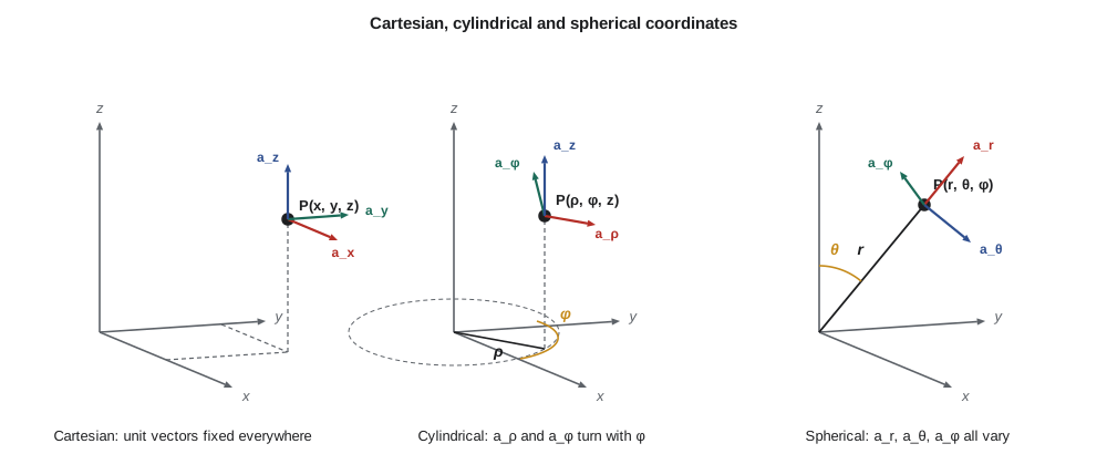
Cartesian coordinates suit flat boundaries such as a printed-circuit board or a slab of concrete. Many electromagnetic problems have other symmetries, and choosing coordinates that match the symmetry turns hard integrals into easy ones. Cylindrical coordinates (ρ, φ, z) suit long straight wires and coaxial cables: ρ is the distance from the z axis, φ the angle around it measured from the x axis, and z the height. Spherical coordinates (r, θ, φ) suit point charges and antennas: r is the distance from the origin, θ the angle down from the z axis, and φ the same azimuth as in cylindrical coordinates. A dipole antenna is described almost entirely by θ, so its radiation pattern is drawn in spherical coordinates.
| Quantity | Cartesian (x, y, z) | Cylindrical (ρ, φ, z) | Spherical (r, θ, φ) |
|---|---|---|---|
| From Cartesian | — | ρ = √(x² + y²), φ = atan2(y, x), z = z | r = √(x² + y² + z²), θ = arccos(z/r), φ = atan2(y, x) |
| To Cartesian | — | x = ρ cos φ, y = ρ sin φ | x = r sin θ cos φ, y = r sin θ sin φ, z = r cos θ |
| Differential length | dx a_x + dy a_y + dz a_z | dρ a_ρ + ρ dφ a_φ + dz a_z | dr a_r + r dθ a_θ + r sin θ dφ a_φ |
| Differential volume | dx dy dz | ρ dρ dφ dz | r² sin θ dr dθ dφ |
| Natural for | Boards, slabs, waveguides | Wires, coaxial cable, loops seen from the axis | Point charges, antennas, far fields |
One subtlety catches many students. In Cartesian coordinates the unit vectors are the same everywhere. In cylindrical and spherical coordinates they are not: a_ρ at a point on the positive x axis points along +x, but at a point on the positive y axis it points along +y. So you cannot add two vectors written in cylindrical components at different points by adding their components. Convert both to Cartesian components first, or add them only when they are defined at the same point. Integrals that contain a_ρ or a_r must likewise have those unit vectors expressed in Cartesian form before integrating, unless symmetry makes the varying parts cancel.
Worked problem
Locating the far-pole antenna
At an intersection, the TLR-1 cabinet antenna is at the origin. The antenna on the far pole is 38.0 m east, 24.0 m north and 3.5 m lower. Amara wants its cylindrical and spherical coordinates, because antenna patterns are specified in spherical coordinates about the antenna's own axis.
Show solution
- \[\rho = \sqrt{38.0^2 + 24.0^2} = 44.94\ \text{m} \qquad \phi = \operatorname{atan2}(24.0,\ 38.0) = 32.3^\circ\]
- \[r = \sqrt{38.0^2 + 24.0^2 + 3.5^2} = 45.08\ \text{m}\]
- \[\theta = \arccos\frac{-3.5}{45.08} = 94.5^\circ\]
- The far antenna lies 4.5° below the horizontal plane through the cabinet antenna, so a vertical dipole at the cabinet sends it almost exactly its peak horizontal gain.
Answer: Cylindrical (44.94 m, 32.3°, −3.5 m); spherical (45.08 m, 94.5°, 32.3°). The distance used in the ELE-350 link budget, about 45 m, is the spherical r.
Line, surface and volume integrals
Three kinds of integral recur. A line integral ∫ A·dl adds up the component of a field along a path; the work done on a unit charge by the electric field from a to b is ∫ E·dl, and its negative is the potential difference. When the path closes on itself we write ∮ and call the result the circulation. A surface integral ∫ A·dS adds up the component of a field normal to a surface; this is the flux, such as the magnetic flux through a loop of wire, which lesson 5 will connect to induced voltage. A volume integral ∫ ρ_v dv adds up a scalar density, such as the total charge in a region with charge density ρ_v.
The differential elements in the table make these integrals concrete. On a cylinder of radius ρ, a small patch of surface has area ρ dφ dz and points along a_ρ. On a sphere of radius r, a patch has area r² sin θ dθ dφ and points along a_r. The factor ρ or r² sin θ is exactly what makes the total come out right: integrating r² sin θ dθ dφ over a full sphere gives 4πr², and integrating ρ dφ dz around a cylinder of length L gives 2πρL. Many results in lessons 2 to 4, such as the field of a line charge or the field inside a coaxial cable, follow in two lines once the right surface is chosen.
Gradient, divergence and curl
The del operator ∇ = a_x ∂/∂x + a_y ∂/∂y + a_z ∂/∂z produces three operations. The gradient ∇V of a scalar field points in the direction in which V increases fastest, and its magnitude is that rate of increase. Equipotential surfaces are everywhere perpendicular to the gradient. In lesson 2 you will see that the electric field is simply E = −∇V: field lines run downhill on the potential landscape, at right angles to the equipotentials.
The divergence ∇·A of a vector field is a scalar that measures how much the field spreads out from a point, the net outward flux per unit volume of a tiny closed surface. A positive divergence marks a source, a negative divergence a sink, and zero divergence means whatever flows in also flows out. Gauss's law states that the divergence of the electric flux density equals the charge density, ∇·D = ρ_v, and the magnetic field always has zero divergence, ∇·B = 0, because there are no magnetic charges.
The curl ∇×A of a vector field is a vector that measures circulation: the circulation per unit area round a tiny loop, with direction normal to the loop that gives the largest value. A field with zero curl everywhere is called conservative or irrotational, and the line integral between two points does not depend on the path. Static electric fields are like that. Magnetic fields curl around currents, ∇×H = J, and a changing magnetic field makes the electric field curl, which is Faraday's law. The Laplacian ∇²V = ∇·∇V combines gradient and divergence and appears in Poisson's and Laplace's equations, which govern potentials in charge-free regions such as the air between conductors.
In cylindrical and spherical coordinates the operators have extra factors, because the unit vectors and the differential lengths change from point to point. You do not need to memorize them; every textbook prints them inside the cover, and you should keep a copy beside you. What you should remember is the meaning: gradient is the steepest slope, divergence is outflow per unit volume, curl is circulation per unit area.
The divergence theorem and Stokes' theorem
Two theorems connect the differential operators with integrals. The divergence theorem says that the total outward flux of a field through a closed surface equals the volume integral of its divergence inside: the net amount leaving equals the sum of all the sources inside. Stokes' theorem says that the circulation of a field round a closed path equals the flux of its curl through any surface bounded by the path. Each of Maxwell's equations has a differential form, true at a point, and an integral form, true for a region; these two theorems convert one into the other.
The integral forms are often more useful in engineering. Gauss's law in integral form lets you find the field of a symmetric charge distribution by choosing a closed surface on which the field is constant. Ampère's law in integral form gives the magnetic field of a wire by choosing a circle round it. Faraday's law in integral form tells you the voltage induced in a loop from the flux through it, which is exactly how the loop detector senses a car. The Python block checks both theorems numerically for simple fields, a habit worth keeping whenever you derive something by hand.
import math
# 1. Coordinate conversions for the far-pole antenna seen from the cabinet antenna
x, y, z = 38.0, 24.0, -3.5          # m east, north and up
rho = math.hypot(x, y); phi = math.degrees(math.atan2(y, x))
r = math.sqrt(x*x + y*y + z*z); theta = math.degrees(math.acos(z / r))
print(f"cylindrical: rho = {rho:.2f} m, phi = {phi:.1f} deg, z = {z:.1f} m")
print(f"spherical:   r = {r:.2f} m, theta = {theta:.1f} deg, phi = {phi:.1f} deg")

# 2. Divergence theorem for F = (x^2 y, y z, x z^2) on the unit cube
def F(x, y, z): return (x*x*y, y*z, x*z*z)
def div(x, y, z): return 2*x*y + z + 2*x*z
n = 40; h = 1.0 / n
vol = sum(div((i+.5)*h, (j+.5)*h, (k+.5)*h) for i in range(n) for j in range(n) for k in range(n)) * h**3
flux = 0.0
for i in range(n):
    for j in range(n):
        a, b = (i+.5)*h, (j+.5)*h
        flux += (F(1, a, b)[0] - F(0, a, b)[0]) * h*h      # faces x = 1 and x = 0
        flux += (F(a, 1, b)[1] - F(a, 0, b)[1]) * h*h      # faces y = 1 and y = 0
        flux += (F(a, b, 1)[2] - F(a, b, 0)[2]) * h*h      # faces z = 1 and z = 0
print(f"volume integral of div F = {vol:.4f}, net outward flux = {flux:.4f}, exact 3/2")

# 3. Stokes' theorem: circulation of A = (-y, x, 0) round a circle of radius 0.5 m
N = 2000; R = 0.5; circ = 0.0
for k in range(N):
    t = 2*math.pi*k/N; dt = 2*math.pi/N
    xx, yy = R*math.cos(t), R*math.sin(t)
    dx, dy = -R*math.sin(t)*dt, R*math.cos(t)*dt
    circ += -yy*dx + xx*dy
print(f"circulation = {circ:.5f}, flux of curl (2 x area) = {2*math.pi*R*R:.5f}")cylindrical: rho = 44.94 m, phi = 32.3 deg, z = -3.5 m spherical: r = 45.08 m, theta = 94.5 deg, phi = 32.3 deg volume integral of div F = 1.5000, net outward flux = 1.5000, exact 3/2 circulation = 1.57080, flux of curl (2 x area) = 1.57080
The first part reproduces the coordinates in the worked example. The second part approximates both sides of the divergence theorem for the field F = x²y a_x + yz a_y + xz² a_z on a unit cube, using the midpoint rule on a 40 × 40 × 40 grid. The divergence is 2xy + z + 2xz, whose integral over the cube is exactly 3/2, and the flux through the six faces agrees to four decimals. The third part integrates the field A = −y a_x + x a_y round a circle. Its curl is 2 a_z everywhere, so the flux of the curl through the disc is twice the disc's area, π/2 ≈ 1.5708, and the circulation matches. Small numerical checks like these catch sign errors and missing factors of ρ or r² sin θ long before they reach a design.
Fields as pictures
Engineers think about fields in pictures as much as in symbols. A field-line plot draws curves whose tangent at each point is the field direction, packed closely where the field is strong. Electric field lines begin on positive charges and end on negative ones, and they meet conductors at right angles. Magnetic field lines form closed loops round currents. An equipotential plot draws contours of V, and in a static field the field lines cross the equipotentials at right angles. A good sketch of both tells you where the field is strongest, which is where insulation breaks down, where an electrostatic discharge will jump and where a sensing loop is most sensitive.
Amara keeps a notebook of such sketches for the products. The button cap of the APS-2 is a metal disc 50 mm across in a plastic bezel; she sketches the field lines from a charged finger converging on its edge. The loop detector is a square of wire in a saw cut; she sketches the magnetic field lines rising out of the pavement inside the loop and returning outside it. The TLR-1 antenna is a quarter-wave whip on a metal enclosure; she sketches the field lines that detach from it each half cycle and travel away as a wave. By the end of the course, each sketch will have a calculation behind it.
Units and constants
Electromagnetics uses SI units throughout, in Canada and the United States alike. Two constants define the vacuum. The permittivity of free space ε₀ ≈ 8.854 × 10⁻¹² F/m sets how much electric flux a charge produces, and the permeability μ₀ ≈ 4π × 10⁻⁷ H/m (more precisely 1.256 637 × 10⁻⁶ H/m since the 2019 redefinition of the SI) sets how much magnetic flux a current produces. Together they fix the speed of light, c = 1/√(μ₀ε₀) ≈ 2.998 × 10⁸ m/s, and the impedance of free space, η₀ = √(μ₀/ε₀) ≈ 376.7 Ω. Materials modify these through the relative permittivity ε_r and relative permeability μ_r. Keep track of units in every calculation: the electric field is in volts per meter, the magnetic field H in amperes per meter, the flux density B in teslas and power density in watts per square meter.
Common mistakes
MistakeAdding cylindrical or spherical components of vectors at different points.
InsteadUnit vectors a_ρ, a_φ, a_r and a_θ change direction with position; convert to Cartesian components first.
MistakeForgetting the scale factors ρ and r² sin θ in surface and volume elements.
InsteadUse dS = ρ dφ dz on a cylinder and r² sin θ dθ dφ on a sphere; the factors make areas and volumes correct.
MistakeReversing the vector R in a field formula.
InsteadR = r − r′ points from the source to the field point.
MistakeTreating the curl or divergence as numbers without units.
Instead∇ has units of 1/m: ∇·D is in C/m³, ∇×H in A/m², ∇V in V/m.
Summary and key terms
- Electromagnetic fields are vector fields described with vector calculus; circuit theory is a special case for small structures.
- The dot product picks out the component of one vector along another; the cross product gives a vector perpendicular to both.
- Choose Cartesian, cylindrical or spherical coordinates to match the geometry; remember that curvilinear unit vectors vary with position.
- Line integrals give work and circulation, surface integrals give flux, volume integrals give totals such as charge.
- Gradient is the steepest slope of a scalar, divergence the outflow per unit volume, curl the circulation per unit area.
- The divergence theorem and Stokes' theorem link the differential and integral forms of Maxwell's equations.
- Vector field
- A function that assigns a vector, such as E or H, to every point in a region.
- Position vector
- The vector from the origin to a point; R = r − r′ runs from a source point to a field point.
- Flux
- The surface integral of the normal component of a field through a surface.
- Circulation
- The line integral of a field round a closed path.
- Gradient
- The vector ∇V giving the direction and rate of fastest increase of a scalar field.
- Divergence
- The scalar ∇·A giving the net outward flux per unit volume at a point.
- Curl
- The vector ∇×A giving the circulation per unit area and its axis at a point.
- Divergence theorem
- The flux through a closed surface equals the volume integral of the divergence inside it.
- Stokes' theorem
- The circulation round a closed path equals the flux of the curl through a surface it bounds.
Practice problems
Work each problem on paper first, then reveal the answer to check.
Find A·B and A×B for A = 3a_x − 2a_y + a_z and B = a_x + 4a_y − 2a_z.
Show answer
A·B = −7; A×B = 0a_x + 7a_y + 14a_z.
Convert the point (x, y, z) = (−2, 2, 1) m to cylindrical and spherical coordinates.
Show answer
ρ = 2.83 m, φ = 135°; r = 3 m, θ = 70.5°, φ = 135°.
Find the gradient of V = 10x²y − 5z volts at (1, 2, 0) m.
Show answer
∇V = 40a_x + 10a_y − 5a_z V/m.
Find the divergence of D = 2xy a_x + x² a_y + 3z a_z C/m².
Show answer
∇·D = 2y + 3 C/m³.
Use the spherical volume element to find the volume of a sphere of radius a.
Show answer
∫₀^a ∫₀^π ∫₀^{2π} r² sin θ dφ dθ dr = 4πa³/3.
The circulation of a field round a 2 cm square loop is 6 × 10⁻⁴ A, and the curl is uniform and normal to the loop. What is the curl?
Show answer
6 × 10⁻⁴ / (0.02)² = 1.5 A/m², which by Ampère's law is the current density through the loop.
Lesson quiz · 5 questions
Score 60% or more to complete this lesson.
Create a free account to save your progress, take quizzes and earn a certificate.