
ELE-350 · Lesson 7 of 12 · 23 min
Random processes and noise
Noise sets the ultimate limit on every communication system. A receiver can be given more gain, sharper filters and better linearity, but it cannot hear a signal weaker than its own noise without paying in bandwidth, time or power. To design against noise, an engineer must describe it, and because noise is random, the description is statistical. This lesson connects the probability of STAT-235 to signals: random processes, autocorrelation and power spectral density, white and filtered noise, the physical sources of noise, noise figure and noise temperature, the Friis formula for cascaded stages, and receiver sensitivity. It ends with the in-phase and quadrature description of narrowband noise, which the detection analysis of lesson 9 and the fading model of lesson 11 both need.
Amara has a specific decision to make. The SAW filter she added in lesson 4 protects the TLR-1 cabinet receiver from the truck radio and the cellular base stations, but it has 2 dB of insertion loss. Should it go before the transceiver chip's own low-noise amplifier, or should an external LNA come first? The answer comes from the Friis formula at the end of this lesson, and the reasoning applies to every receiver.
Random variables and random processes
A random variable assigns a number to each outcome of an experiment; its behavior is described by a probability density function. The Gaussian, or normal, density is the most important in communication, for a reason rooted in the central limit theorem: thermal noise is the sum of tiny contributions from enormous numbers of electrons, so it is Gaussian to an excellent approximation. A Gaussian variable is fully described by its mean μ and variance σ².
The Q-function, the probability that a standard Gaussian variable exceeds a, has no closed form but is tabulated and easy to compute from the complementary error function, Q(a) = ½ erfc(a/√2). Q(3) is about 1.35 × 10⁻³ and Q(4.75) is about 1 × 10⁻⁶; lesson 9 relies on these numbers.
A random process is a random function of time, such as the noise voltage across a resistor. At any one instant its value is a random variable. A process is stationary if its statistics do not change with time, and ergodic if time averages along one sample function equal averages across the ensemble of possible functions. Noise in a receiver that has been switched on for a while is both, to good approximation, which lets an engineer measure its statistics with one long recording, exactly as a spectrum analyzer does.
Autocorrelation and power spectral density
The autocorrelation function R(τ) of a stationary process measures how similar the signal is to a shifted copy of itself: the average of x(t)x(t + τ). Its value at τ = 0 is the mean-square value, the average power. The Wiener-Khinchin theorem states that the power spectral density S(f), the distribution of power over frequency, is the Fourier transform of the autocorrelation. A process that changes quickly has a narrow autocorrelation and a wide spectrum, the same duration-bandwidth trade as for deterministic signals.
When a random process passes through a linear filter with frequency response H(f), the output spectral density is the input density times |H(f)|². This simple rule is how every noise calculation in a receiver is done.
White noise and noise bandwidth
White noise has a flat spectral density at all frequencies of interest. By convention its two-sided density is written N₀/2, so that the power in a band of width B, counting both positive and negative frequencies, is N₀B. Its autocorrelation is an impulse: samples at different times, however close, are uncorrelated. Truly white noise would have infinite power, but thermal noise is flat up to frequencies far above any radio band, so the model is excellent.
A real filter does not have a rectangular response, so the noise it passes is described by its noise-equivalent bandwidth B_N, the width of the ideal rectangular filter with the same peak gain that would pass the same noise power. For a single-pole RC low-pass filter with a 3 dB corner f_c, B_N = (π/2)f_c, about 57 percent wider than the 3 dB bandwidth. For sharper filters, B_N is close to the 3 dB bandwidth.
Sources of noise
Thermal noise, or Johnson-Nyquist noise, comes from the random motion of electrons in any conductor above absolute zero. A resistor R at temperature T produces an open-circuit noise voltage with mean-square value 4kTRB in a bandwidth B, where k = 1.38 × 10⁻²³ J/K is Boltzmann's constant. When that resistor is connected to a matched load, the power delivered, the available noise power, is kTB, independent of R. At the standard reference temperature T₀ = 290 K, kT₀ is 4.0 × 10⁻²¹ W/Hz, or −174 dBm/Hz. This number is the starting point of every receiver noise calculation.
Shot noise arises because current in a diode or transistor is a stream of discrete charges crossing a junction at random times; its mean-square current is 2qIB. Flicker, or 1/f, noise grows at low frequencies and matters in audio amplifiers and in the baseband stages of direct-conversion receivers, as lesson 4 noted. Outside the receiver, the antenna collects noise too: thermal radiation from the ground and buildings, cosmic noise from the sky and, in cities at frequencies below about 1 GHz, man-made noise from vehicle ignition, power lines and electronics. An antenna's noise is described by its noise temperature, the temperature of a resistor that would give the same available noise power. A 900 MHz antenna at street level in a city may see a noise temperature well above 290 K at times, a reason to keep a margin in the link budget.
Noise figure and noise temperature
Every amplifier adds noise of its own. The noise factor F of a two-port is the ratio of the input SNR to the output SNR when the input noise comes from a source at 290 K. Its value in dB is the noise figure, NF. A perfect amplifier has F = 1, an NF of 0 dB. An equivalent description is the effective input noise temperature T_e: the amount by which the source temperature would have to rise to account for the amplifier's added noise. The two are related by T_e = (F − 1)T₀. Noise temperature is preferred for very quiet systems such as satellite receivers, where noise figures are a fraction of a decibel.
A passive lossy component at room temperature, such as a cable, a filter or a switch, has a noise factor equal to its loss: a 2 dB filter has a 2 dB noise figure. The loss attenuates the signal, but the component's own thermal noise keeps the noise at the output at the same kT₀B, so the SNR falls by exactly the loss.
Cascaded stages: the Friis formula
A receiver is a chain of stages, each with its own gain G and noise factor F. Friis showed that the noise factor of the whole chain is dominated by the first stage. Each later stage's excess noise, F − 1, is divided by the total gain ahead of it, so a stage behind a high-gain amplifier hardly matters.
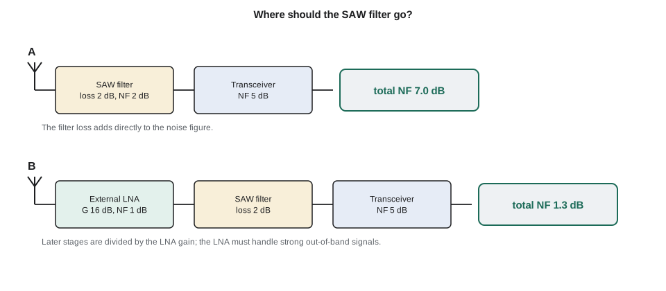
The formula answers Amara's question. With the 2 dB SAW filter ahead of a transceiver whose NF is 5 dB, the chain's noise figure is 2 + 5 = 7 dB, because the filter's loss is in front of everything. With an external LNA of 16 dB gain and 1 dB noise figure placed first, the filter's loss and the chip's noise are both divided by the LNA's gain, and the total noise figure falls to about 1.3 dB, a 5.7 dB improvement in sensitivity. The catch is linearity: the LNA now sees the truck radio and the cellular signals unfiltered, so it needs a high IIP3 and blocking performance. Many designs compromise with a broad, low-loss filter before the LNA and the sharp SAW after it.
Worked problem
Two front-end arrangements
Find the total noise figure of: (A) a SAW filter with 2 dB loss followed by a transceiver with NF = 5 dB; (B) an LNA with G = 16 dB and NF = 1 dB, then the SAW filter, then the transceiver.
Show solution
- \[\text{A: } F = 1.585 + \frac{3.162 - 1}{1/1.585} = 1.585 \times 3.162 = 5.01 \;\Rightarrow\; 7.0\ \text{dB}\]
- \[\text{B: } F = 1.259 + \frac{1.585 - 1}{39.81} + \frac{3.162 - 1}{39.81/1.585} = 1.259 + 0.015 + 0.086 = 1.360\]
- \[\text{NF}_B = 10\log_{10}1.360 \approx 1.33\ \text{dB}\]
Answer: Arrangement B gives about 5.7 dB better sensitivity, which lesson 11 will show is worth roughly a doubling of range in some environments. Amara keeps arrangement A for the pole stations, where range is short and cost matters, and plans arrangement B for the 600 m cabinet-to-cabinet link if the budget needs it.
Receiver sensitivity
Putting these pieces together gives the sensitivity of a receiver: the input signal power at which the SNR in the receiver's noise bandwidth reaches the value the demodulator needs. In dB terms it is a sum, sometimes called the sensitivity equation. The bandwidth term shows the cost of speed: a receiver five times wider has 7 dB more noise.
import math, random
k, T0 = 1.380649e-23, 290.0
print(f"kT0 = {10*math.log10(k*T0/1e-3):.1f} dBm/Hz")
def cascade(stages):                 # stages: list of (gain_dB, nf_dB)
    F, G = 0.0, 1.0
    for i, (g, nf) in enumerate(stages):
        f = 10 ** (nf / 10)
        F = f if i == 0 else F + (f - 1) / G
        G *= 10 ** (g / 10)
    return 10 * math.log10(F)
A = [(-2.0, 2.0), (20.0, 5.0)]
B = [(16.0, 1.0), (-2.0, 2.0), (20.0, 5.0)]
print(f"chain A (SAW first): NF = {cascade(A):.2f} dB")
print(f"chain B (LNA first): NF = {cascade(B):.2f} dB")
for rate, bw in ((10e3, 13.5e3), (50e3, 67.5e3)):
    for nf in (cascade(A), cascade(B)):
        s = -174 + 10 * math.log10(bw) + nf + 10.0
        print(f"{rate/1e3:4.0f} kb/s, B = {bw/1e3:4.1f} kHz, NF = {nf:4.2f} dB: sensitivity = {s:6.1f} dBm (10 dB SNR)")
# Gaussian noise and its envelope: check the Q-function and the Rayleigh law
random.seed(350)
n = [random.gauss(0, 1) for _ in range(200000)]
print(f"P(n > 3 sigma): measured {sum(v > 3 for v in n)/len(n):.5f}, Q(3) = {0.5*math.erfc(3/math.sqrt(2)):.5f}")
env = [math.hypot(n[i], n[i+1]) for i in range(0, len(n), 2)]
for r in (1.0, 2.0, 3.0):
print(f"P(envelope > {r:.0f} sigma): measured {sum(e > r for e in env)/len(env):.4f}, Rayleigh {math.exp(-r*r/2):.4f}")kT0 = -174.0 dBm/Hz chain A (SAW first): NF = 7.00 dB chain B (LNA first): NF = 1.33 dB 10 kb/s, B = 13.5 kHz, NF = 7.00 dB: sensitivity = -115.7 dBm (10 dB SNR) 10 kb/s, B = 13.5 kHz, NF = 1.33 dB: sensitivity = -121.4 dBm (10 dB SNR) 50 kb/s, B = 67.5 kHz, NF = 7.00 dB: sensitivity = -108.7 dBm (10 dB SNR) 50 kb/s, B = 67.5 kHz, NF = 1.33 dB: sensitivity = -114.4 dBm (10 dB SNR) P(n > 3 sigma): measured 0.00134, Q(3) = 0.00135 P(envelope > 1 sigma): measured 0.6056, Rayleigh 0.6065 P(envelope > 2 sigma): measured 0.1342, Rayleigh 0.1353 P(envelope > 3 sigma): measured 0.0112, Rayleigh 0.0111
The sensitivity lines show the two levers Amara holds. Dropping from 50 to 10 kb/s improves sensitivity by 7 dB; adding the external LNA improves it by 5.7 dB. Either choice, or both, can buy range. The Monte Carlo check confirms the Q-function value and a second law that the next section derives.
Narrowband noise
After the IF or channel filter, noise occupies a narrow band around the carrier frequency. Such narrowband noise can be written in the same form as a modulated signal, with slowly varying in-phase and quadrature components n_I(t) and n_Q(t), each a Gaussian low-pass process with the same power as the band-pass noise. Equivalently, it is a sinusoid at f_c with a randomly varying envelope r(t) and phase ψ(t).
Because n_I and n_Q are independent Gaussian variables with equal variance σ², the envelope has a Rayleigh distribution, and the phase is uniformly distributed. The probability that the envelope exceeds r is e^(−r²/2σ²). This result has two uses later in the course. It gives the error rate of non-coherent receivers, which decide by comparing envelopes, in lesson 9. And the same mathematics describes the signal itself when it arrives over many scattered paths with no direct path, Rayleigh fading, in lesson 11.
| Quantity | Symbol | Typical value or rule |
|---|---|---|
| Thermal noise density at 290 K | kT₀ | −174 dBm/Hz |
| Noise in 1 MHz | kT₀B | −114 dBm |
| Noise figure of a passive loss L | NF | equal to L in dB |
| Good discrete LNA at 900 MHz | NF | below 1 dB |
| Integrated sub-GHz transceiver | NF | about 4–7 dB |
| Noise temperature | T_e | (F − 1) × 290 K; NF 1 dB is about 75 K |
Common mistakes
MistakeUsing the 3 dB bandwidth of a gentle filter as its noise bandwidth.
InsteadUse the noise-equivalent bandwidth; for a single pole it is π/2 times the 3 dB bandwidth.
MistakeAdding noise figures in dB down a chain.
InsteadUse Friis with linear factors and gains; only the first stage adds directly.
MistakeForgetting that a filter or cable before the LNA adds its loss to the noise figure.
InsteadLoss at the front degrades the whole chain dB for dB; keep it short or put a good LNA first.
MistakeAssuming the antenna always delivers noise at 290 K.
InsteadMan-made noise in cities can make the effective antenna temperature higher; leave margin.
Summary and key terms
- Thermal noise is Gaussian; the Q-function gives its tail probabilities.
- Power spectral density is the Fourier transform of autocorrelation; through a filter it is multiplied by |H(f)|².
- White noise of density N₀/2 delivers N₀B_N in a noise bandwidth B_N; kT₀ = −174 dBm/Hz.
- Noise factor is the SNR degradation of a stage; a passive loss L has F = L; T_e = (F − 1)T₀.
- Friis: the first stage dominates; later stages are divided by the gain ahead of them.
- Sensitivity = −174 + 10 log B + NF + required SNR; narrowband noise has a Rayleigh envelope.
- Random process
- A random function of time, such as a noise voltage.
- Power spectral density
- The distribution of a signal's power over frequency.
- White noise
- Noise with a flat power spectral density.
- Noise-equivalent bandwidth
- The width of an ideal rectangular filter passing the same noise power as a real filter.
- Thermal noise
- Noise caused by random electron motion in conductors, of available power kTB.
- Noise figure
- The degradation of SNR by a stage, in dB, with a 290 K source.
- Friis formula
- The expression for the noise factor of cascaded stages.
- Rayleigh distribution
- The distribution of the envelope of narrowband Gaussian noise.
Practice problems
Work each problem on paper first, then reveal the answer to check.
Find the thermal noise power in a 200 kHz bandwidth at 290 K.
Show answer
−174 + 53 = −121 dBm.
Convert NF = 3 dB to noise temperature.
Show answer
F = 2, so T_e = 290 K.
An LNA (G = 20 dB, NF = 2 dB) is followed by a mixer with NF = 12 dB. Find the total NF.
Show answer
F = 1.585 + (15.85 − 1)/100 = 1.734, NF ≈ 2.4 dB.
A receiver has B = 25 kHz, NF = 6 dB and needs 12 dB SNR. Find its sensitivity.
Show answer
−174 + 44 + 6 + 12 = −112 dBm.
A single-pole filter has f_c = 10 kHz. What is its noise bandwidth?
Show answer
15.7 kHz.
Narrowband noise has σ = 1 µV per component. What is the probability that its envelope exceeds 3 µV?
Show answer
e^(−4.5) ≈ 0.011.
Lesson quiz · 5 questions
Score 60% or more to complete this lesson.
Create a free account to save your progress, take quizzes and earn a certificate.