Link budgets, propagation and fading

A link budget is the accounting sheet of a radio link. It starts with the transmitter's power, adds the antenna gains, subtracts every loss along the way, and compares the result with the receiver's sensitivity. The difference is the margin, and it must be large enough to cover what the simple calculation leaves out: obstructions, reflections, fading and the noise of a busy city. This lesson builds the link budget from the Friis transmission equation, explains free-space and ground-reflection propagation, the Fresnel zone, log-distance models and shadowing, and then the multipath fading that makes mobile and urban links so variable, with the fade margins and diversity techniques that tame it.

Leo has spent two days with a test transmitter and a spectrum analyzer at the first pilot intersection. His notes show what textbooks warn about: the signal across the intersection is steady most of the time, but each time a bus stops between the pole and the cabinet it drops by 10 to 20 dB, and at a few positions of the receiving antenna the level is 15 dB lower than a few centimeters away. Amara needs to turn those observations into numbers for the design.

The Friis transmission equation

In free space, a transmitter radiating power P_t equally in all directions spreads it over a sphere of area 4πd² at distance d. An antenna with gain G_t concentrates the power in its preferred direction, and the product P_tG_t is the effective isotropic radiated power (EIRP). A receiving antenna collects power in proportion to its effective aperture A_e = G_rλ²/4π. Combining these gives the Friis equation, and its logarithmic form is the backbone of every link budget.

Free-space path loss grows 20 dB per decade of distance, 6 dB for each doubling, and 20 dB per decade of frequency. The frequency dependence is not because high frequencies are absorbed in free space; it reflects the smaller aperture of an antenna of fixed gain at a shorter wavelength. At 915 MHz the loss is 31.7 dB at 1 m, 64.7 dB at 45 m and 87.2 dB at 600 m.

Building a link budget

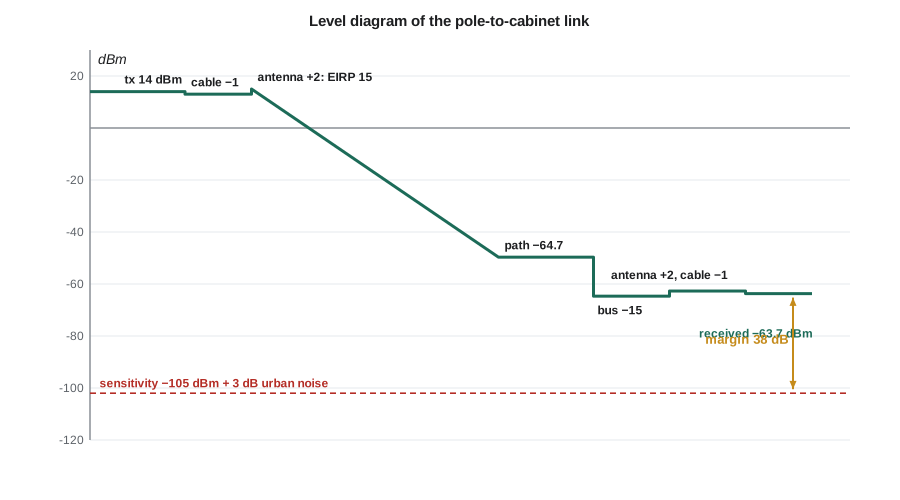
A link budget is written as a column of gains and losses in dB. A typical form: transmitter output power, minus transmitter cable and connector losses, plus transmit antenna gain gives EIRP; minus path loss and any extra losses, such as obstructions or body loss; plus receive antenna gain, minus receive cable losses gives received power. The receiver sensitivity, from lesson 9, is subtracted to give the link margin. Each line should state its assumptions, because the margin is only as good as the weakest of them.

Ground reflection and the two-ray model

Near the ground, the receiver sees the direct wave and a wave reflected from the road surface. For grazing angles the reflection coefficient is close to −1, so the two waves cancel more and more as the distance grows and the path difference shrinks. Up to a breakpoint distance the received power oscillates around the free-space value; beyond it, it falls as 1/d⁴, 40 dB per decade, and becomes independent of frequency. Raising either antenna pushes the breakpoint out. This is why point-to-point links are mounted as high as practical, and why the TLR-1's cabinet-to-cabinet antennas will go on the signal mast arms rather than on the cabinets.

The Fresnel zone

A radio wave does not travel along a line; the energy that reaches the receiver flows through an ellipsoidal region around the direct path. The first Fresnel zone is the region where path lengths differ from the direct path by less than half a wavelength. If an obstacle intrudes into it, the received power drops even though the antennas can still see each other. A common rule keeps at least 60 percent of the first Fresnel zone clear. Its radius at a point d₁ from one end and d₂ from the other, on a path of length d, is

For the 600 m cabinet link at 915 MHz, the radius at mid-path is about 7 m. Antennas 6 m high on mast arms over a street lined with parked trucks and buses do not clear it, so the link will see some obstruction loss even on a clear day. Raising the antennas helps, and so does accepting it in the budget.

Path-loss models and shadowing

Real environments are neither free space nor a flat plane. Empirical models describe the average loss with a log-distance law: loss rises 10n dB per decade beyond a reference distance d₀, with a path-loss exponent n of about 2 in free space, 2.7 to 3.5 in urban areas and up to 4 to 6 in dense obstruction. Around that average, the actual loss at a particular location varies because buildings, trees and vehicles shadow some places more than others. Measurements show that this shadowing is roughly Gaussian in dB, called log-normal shadowing, with a standard deviation σ of about 6 to 10 dB in cities. Models such as Okumura-Hata and its extensions give curves for typical cities, suburbs and open areas from extensive measurements, and planning software applies them with terrain and building data.

Shadowing explains Leo's bus. A bus between the antennas adds a loss of 10 to 20 dB that lasts for the 20 or 30 seconds the bus is stopped. It is slow, it is large and it cannot be averaged away within one packet. The design must either carry enough margin for it or provide another path.

Multipath fading

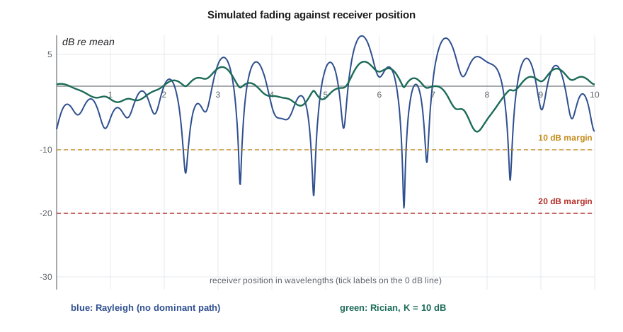
Leo's second observation, deep drops a few centimeters apart, has a different cause. In a city the signal arrives over many paths at once, reflected from buildings, vehicles and poles, each with its own amplitude, phase and delay. They add as phasors, and where they cancel the signal fades deeply. Moving half a wavelength, 16 cm at 915 MHz, changes the phase relations completely, so the fades are spaced roughly every half-wavelength. When no path dominates, the in-phase and quadrature sums are Gaussian by the central limit theorem, so the envelope has exactly the Rayleigh distribution derived for narrowband noise in lesson 7. When one path, usually line of sight, is strong, the distribution is Rician, characterized by the K factor, the ratio of the dominant power to the scattered power.

Rayleigh fading is severe. The probability that the power falls 10 dB below its average is about 10 percent; 20 dB, 1 percent; 30 dB, 0.1 percent. A link with a fixed margin F against the average is therefore unavailable a fraction about 1/F of the time or locations. Achieving 99.9 percent availability against Rayleigh fading takes a 30 dB fade margin, a huge price in power. With a strong line of sight, a Rician K of 6 to 10 dB, the required margin is much smaller.

Delay spread, coherence bandwidth and Doppler

Multipath also spreads the signal in time. The RMS delay spread τ_rms measures how long the echoes last; it ranges from tens of nanoseconds indoors to a few microseconds in a hilly city. Its inverse sets the coherence bandwidth, the frequency range over which the channel fades together: roughly B_c ≈ 1/(5τ_rms). If the signal is narrower than B_c, the whole signal fades up and down together, flat fading. If it is wider, different parts of the spectrum fade differently and the echoes cause intersymbol interference, frequency-selective fading, which needs an equalizer or OFDM. Motion changes the channel in time: the Doppler spread f_D = v/λ sets how fast, and the coherence time, roughly 0.4/f_D, is how long the channel stays nearly constant.

For the TLR-1 across an intersection, a delay spread of a few hundred nanoseconds gives a coherence bandwidth of several hundred kilohertz, much wider than the 75 kHz signal, so fading is flat: the eye stays open, but the whole signal fades. A bus moving at 10 m/s near the path gives a Doppler spread of about 30 Hz and a coherence time of about 14 ms, longer than a 5 ms packet, so each packet sees a nearly constant channel. Those two facts shape the design: no equalizer is needed, but a packet sent in a fade will fail, and an immediate retry may fail too unless something changes.

Diversity

The remedy for deep, independent fades is diversity: send or receive the signal through two or more paths that are unlikely to fade at the same time. With two independent branches and selection of the stronger, the probability that both are in a 20 dB fade is 0.01 × 0.01 = 10⁻⁴ instead of 10⁻², which lowers the required margin dramatically. Space diversity uses antennas spaced at least about half a wavelength apart at the mobile, more at a base station. Frequency diversity sends on frequencies farther apart than the coherence bandwidth, and frequency hopping provides it automatically: each retry on a new channel several megahertz away sees an almost independent fade. Time diversity sends again after more than the coherence time, which is what spreading retries over tens of milliseconds achieves. OFDM, used by Wi-Fi, LTE and digital broadcasting, divides a wide signal into many narrow subcarriers, each narrower than the coherence bandwidth so each fades flatly, and combines it with coding and interleaving across subcarriers, turning frequency-selective fading into a diversity advantage.

import math, random
f = 915e6; lam = 3e8 / f
fspl = lambda d: 20 * math.log10(4 * math.pi * d / lam)
for d in (1, 45, 600):
    print(f"free-space loss at {d:4d} m: {fspl(d):5.1f} dB")
for ht, hr, name in ((3.0, 2.5, 'pole to cabinet'), (6.0, 6.0, 'mast arm to mast arm')):
    print(f"two-ray breakpoint, {name} ({ht} m, {hr} m): {4*ht*hr/lam:.0f} m")
r1 = math.sqrt(lam * 300 * 300 / 600)
print(f"first Fresnel radius at mid-path of 600 m: {r1:.1f} m (60 % clearance: {0.6*r1:.1f} m)")
for p in (0.1, 0.01, 0.001):
    print(f"Rayleigh: margin for {100*(1-p):.1f} % availability = {10*math.log10(-1/math.log(1-p)):.1f} dB")
random.seed(11)
def rayleigh():                                   # power relative to mean, one sample
    return random.gauss(0, 1) ** 2 / 2 + random.gauss(0, 1) ** 2 / 2
n = 200000
for margin_db in (10, 20):
    th = 10 ** (-margin_db / 10)
    one = sum(rayleigh() < th for _ in range(n)) / n
    two = sum(max(rayleigh(), rayleigh()) < th for _ in range(n)) / n
    print(f"{margin_db} dB margin: outage one branch {one:.4f}, two-branch selection {two:.5f}")
v = 10.0; fd = v / lam
print(f"Doppler at {v} m/s: {fd:.1f} Hz, coherence time about {0.423/fd*1e3:.0f} ms")

free-space loss at    1 m:  31.7 dB
free-space loss at   45 m:  64.7 dB
free-space loss at  600 m:  87.2 dB
two-ray breakpoint, pole to cabinet (3.0 m, 2.5 m): 92 m
two-ray breakpoint, mast arm to mast arm (6.0 m, 6.0 m): 439 m
first Fresnel radius at mid-path of 600 m: 7.0 m (60 % clearance: 4.2 m)
Rayleigh: margin for 90.0 % availability = 9.8 dB
Rayleigh: margin for 99.0 % availability = 20.0 dB
Rayleigh: margin for 99.9 % availability = 30.0 dB
10 dB margin: outage one branch 0.0949, two-branch selection 0.00879
20 dB margin: outage one branch 0.0100, two-branch selection 0.00012
Doppler at 10.0 m/s: 30.5 Hz, coherence time about 14 ms

The program confirms the earlier figures and shows the power of diversity: with a 10 dB margin, one branch is out about 9.5 percent of the time, while two independent branches with selection are out less than 1 percent of the time, roughly the square. With a 20 dB margin, two branches reach about one in ten thousand. The pole-to-cabinet breakpoint of about 92 m lies beyond the 45 m path, so the across-intersection link behaves roughly like free space plus obstructions, while the 600 m cabinet link lies beyond its breakpoint of about 440 m and will lose more than free space predicts.