
ELE-350 · Lesson 1 of 12 · 27 min
Communication systems and signals
A communication system moves information from one place to another through a medium that was never designed to carry it cleanly. A voice crosses a city on a radio wave, a sensor reading crosses a parking lot on a 915 MHz signal, and a bank of telephone calls shares one optical fiber. In every case the information has to be turned into a signal that suits the medium, it is weakened, distorted and corrupted with noise on the way, and the receiver has to recover the original message as faithfully as the design allows. This course studies how that is done: how analog and digital messages are placed onto carriers, how noise sets the limits, how receivers are built and how much information a channel can carry at all.
Cedarline Controls in Madison has a new project that will run through the whole course. The city wants to add accessible pedestrian signals and new detectors at intersections where cutting a trench for interconnect cable would mean closing a busy street on the isthmus for weeks. Daniel Fortin, PE, has asked Amara Osei to lead the radio side of the TLR-1 telemetry radio: a small 900 MHz transceiver in each APS-2 push-button station and detector pole that reports button presses, status and faults to the controller cabinet, plus a longer link that lets the cabinet coordinate with the next intersection along the street. Leo Tremblay, the co-op student, will build test fixtures and take most of the measurements.
The requirements Daniel hands over are short. Each pole station must deliver a button press to the cabinet in under 100 ms, with fewer than one lost message in a million, across about 45 m of intersection that includes buses, trucks and steel poles. The cabinet-to-cabinet link must cover 600 m along the street. Everything must run in a license-exempt band, survive winter and summer cabinet temperatures, and never interfere with anyone else. Before Amara can choose a modulation or an antenna, she needs a common vocabulary for signals, bandwidth and power, which is what this first lesson provides.
The elements of a communication system
Every communication system, from a smoke signal to a cellular network, can be drawn with the same blocks. The source produces the message: a voice, a temperature, a button press. An input transducer turns the message into an electrical baseband signal, the message signal m(t), whose spectrum sits near zero frequency. The transmitter processes that signal so it suits the channel; for a radio link this means modulation onto a carrier, filtering and power amplification. The channel is the physical path: a pair of wires, a coaxial cable, an optical fiber or free space between two antennas. The receiver filters, amplifies, demodulates and decides, and an output transducer delivers the message to its destination, the sink.
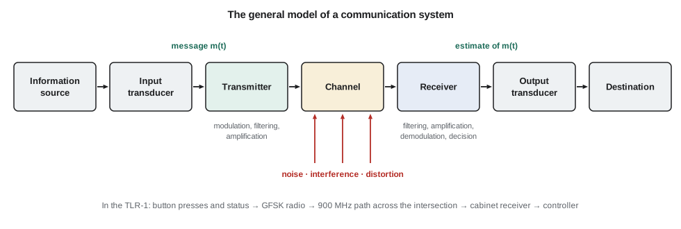
Three kinds of impairment are drawn entering the channel. Distortion is a change in the shape of the signal caused by the channel itself: a cable that attenuates high frequencies more than low ones, a filter whose delay varies with frequency, or an amplifier driven into saturation. Linear distortion can in principle be undone by an equalizer, because the channel's effect is known and repeatable. Interference is an unwanted signal from another man-made source, such as a neighbor's transmitter or a switching power supply, and it can be reduced by filtering, by choosing frequencies and by shielding. Noise is random: thermal agitation of electrons in every resistor, shot noise in semiconductors, and natural radio noise from the sky. Noise can never be removed, only made small compared with the signal, and the ratio between the two, the signal-to-noise ratio, is the single number that most often decides whether a link works.
Analog and digital messages
An analog message can take any value in a continuous range, like a microphone voltage. A digital message is a sequence of symbols from a finite alphabet, like the bytes of a status report. The distinction matters because the receiver's job differs. An analog receiver tries to reproduce a waveform, and every bit of noise that reaches the output degrades it; quality is measured by output signal-to-noise ratio. A digital receiver only has to decide which of a few symbols was sent, and if the noise is small enough, it decides correctly and the noise disappears completely. Quality is measured by the probability of a wrong decision, the bit error rate. That is why a digital signal can be regenerated over and over along a long path, while an analog signal accumulates noise at every repeater.
Most modern systems are digital even when the message is analog: a voice is sampled and quantized into bits, the bits are sent, and the voice is rebuilt at the far end. Lessons 5 and 6 cover that conversion and the transmission of the resulting pulses. The analog modulation methods of lessons 2 to 4 remain important, though. Broadcast radio, aviation voice and many two-way radios still use them, and the ideas they introduce, sidebands, bandwidth, mixing and the superheterodyne receiver, are exactly what a digital radio uses inside.
Why modulate?
The TLR-1 messages are baseband data, a few kilobits per second of ones and zeros. They could in principle drive an antenna directly, but three problems stop that. The first is antenna size. An antenna radiates efficiently when its length is a sizable fraction of a wavelength, and the wavelength is λ = c/f. At 1 kHz the wavelength is 300 km. At 915 MHz it is 32.8 cm, so a quarter-wave whip is about 8 cm long and fits inside a push-button housing. The second is sharing. Many users want to use the radio spectrum at the same time and place; shifting each one to a different carrier frequency lets them coexist, which is frequency-division multiplexing. The third is matching the channel. A channel passes some frequencies well and others badly, and modulation moves the message to where the channel is good and where regulations allow transmission.
Modulation means varying some property of a high-frequency carrier, usually a sinusoid A_c cos(2πf_c t + φ), in step with the message. Varying the amplitude gives amplitude modulation; varying the phase or frequency gives angle modulation; varying them together in discrete steps gives the digital schemes of lesson 8, such as QAM. Demodulation is the reverse process at the receiver.
The radio spectrum and who controls it
Radio spectrum is a shared public resource, and every country controls its use. In the United States, the Federal Communications Commission (FCC) regulates non-federal use, publishes the Table of Frequency Allocations together with the National Telecommunications and Information Administration, and sets equipment rules in Title 47 of the Code of Federal Regulations. Part 15 of those rules lets unlicensed devices operate without a station license if they meet strict power and emission limits. The 902 to 928 MHz band, available for this purpose in the Americas (ITU Region 2), is one of the bands used this way, and it is where the TLR-1 will operate. Lesson 12 returns to the rules an unlicensed device must meet before it can be marketed.
| Service or band | Typical frequencies | Wavelength | Typical use |
|---|---|---|---|
| AM broadcast | 0.53–1.7 MHz | 180–570 m | Medium-wave voice and music |
| FM broadcast | 88–108 MHz | about 3 m | Wideband FM music and data |
| Land mobile radio | 150–170 MHz, 450–470 MHz | 0.65–2 m | Municipal and utility voice and data |
| 900 MHz ISM band | 902–928 MHz | about 33 cm | License-exempt telemetry, meters, sensor networks |
| 2.4 GHz ISM band | 2.400–2.4835 GHz | about 12.5 cm | Wi-Fi, Bluetooth, many short-range devices |
| Cellular | about 0.6–4 GHz and higher | 7–50 cm | Licensed mobile voice and data |
Decibels
Communication engineers work in decibels because signal levels span enormous ranges. A transmitter may put out 0.1 W and the receiver may detect a billionth of a billionth of that. The decibel expresses a power ratio on a logarithmic scale, so that multiplying gains becomes adding numbers. A ratio of voltages across equal resistances uses 20 log₁₀ because power goes as voltage squared. Absolute levels are written relative to a reference: dBm is relative to 1 mW and dBW to 1 W, so 0 dBm is 1 mW, 20 dBm is 100 mW and 30 dBm is 1 W. Antenna gain relative to an ideal isotropic radiator is written dBi.
| Power ratio | dB | Rule of thumb |
|---|---|---|
| 2 | 3.01 | Doubling power adds 3 dB |
| 10 | 10 | Each factor of 10 adds 10 dB |
| 0.5 | −3.01 | Halving power subtracts 3 dB |
| 100 | 20 | 20 dB is a factor of 100 |
| 1 000 000 | 60 | Six factors of ten |
| 10⁻¹² | −120 | A typical path loss over a few hundred meters at 900 MHz |
Worked problem
A level chain in dB
Leo's test transmitter puts out 10 mW into a 2 dB cable, a 3 dBi antenna, a path with 70 dB of loss, a 3 dBi receiving antenna and another 2 dB of cable. Find the received power in dBm and in watts.
Show solution
- \[P_t = 10\log_{10}(10) = 10\ \text{dBm}\]
- \[P_r = 10 - 2 + 3 - 70 + 3 - 2 = -58\ \text{dBm}\]
- \[P_r = 10^{-58/10}\ \text{mW} = 1.58\times10^{-6}\ \text{mW} = 1.58\ \text{nW}\]
Answer: The received power is −58 dBm, about 1.6 nW. Working in dB turns six multiplications into one line of additions and subtractions, and it is how every link budget in lessons 11 and 12 is written.
Signals in time and frequency
Lesson ELE-250 introduced the Fourier transform, which describes a signal as a sum of sinusoids. For communication work, the most important consequence is the trade between duration and bandwidth. A short pulse has a wide spectrum and a long pulse a narrow one. A rectangular pulse of width T has the spectrum T sinc(fT), whose main lobe extends to the first nulls at ±1/T. Sending data faster means shorter pulses, which means a wider band. That single fact links bit rate to bandwidth throughout the course.
A second consequence is the modulation theorem. Multiplying a signal by cos(2πf_c t) shifts its spectrum up and down by f_c, creating two copies centered on ±f_c with half the amplitude. Every modulator in this course is built on that shift, and every demodulator undoes it.
What is bandwidth?
Bandwidth sounds precise, but a real signal's spectrum never stops exactly. Engineers use several definitions, and a specification must say which. The 3 dB bandwidth is the range over which the power spectral density stays within half its peak. The null-to-null bandwidth is the width of the main lobe, 2/T for a rectangular pulse at radio frequency. The 99 percent power bandwidth, often called the occupied bandwidth, contains 99 percent of the total power; regulators use this one or a related 20 dB or 6 dB bandwidth, measured with a spectrum analyzer according to a test procedure. For a signal made of rectangular pulses, the main lobe holds about 90 percent of the power, so the 99 percent bandwidth is several times wider. That is why real transmitters shape their pulses, as lesson 6 shows.
import math
def dbm(p_w): return 10 * math.log10(p_w / 1e-3)
def watts(p_dbm): return 1e-3 * 10 ** (p_dbm / 10)
for p in (1e-3, 10e-3, 0.1, 1.0):
    print(f"{p*1e3:7.1f} mW = {dbm(p):5.1f} dBm")
chain = [('transmitter', 10), ('tx cable', -2), ('tx antenna', 3), ('path', -70), ('rx antenna', 3), ('rx cable', -2)]
level = 0
for name, g in chain:
    level += g
    print(f"after {name:11s}: {level:6.1f} dBm")
print(f"received power = {watts(level)*1e9:.2f} nW")
# fraction of a rectangular pulse's energy inside |f| < k/T (numerical integration of sinc^2)
def frac(k, n=200000):
    h = k / n; s = 0.0
    for i in range(n):
        x = (i + 0.5) * h
        s += (math.sin(math.pi * x) / (math.pi * x)) ** 2
    return 2 * s * h
for k in (1, 2, 3):
print(f"power within |f| < {k}/T: {100*frac(k):.1f} %")1.0 mW = 0.0 dBm 10.0 mW = 10.0 dBm 100.0 mW = 20.0 dBm 1000.0 mW = 30.0 dBm after transmitter: 10.0 dBm after tx cable : 8.0 dBm after tx antenna : 11.0 dBm after path : -59.0 dBm after rx antenna : -56.0 dBm after rx cable : -58.0 dBm received power = 1.58 nW power within |f| < 1/T: 90.3 % power within |f| < 2/T: 95.0 % power within |f| < 3/T: 96.6 %
The output confirms the example and shows the slow decay of the sinc spectrum: one lobe on each side holds about 90 percent of the power, two lobes about 95 percent, and three lobes still not 97 percent. A transmitter that sent rectangular pulses would splash power into neighboring channels, which regulators and neighbors do not allow.
Signal power, noise and SNR
For a periodic or random signal, the useful measure is average power: the mean of x²(t) over a long time, in watts when x is a voltage across 1 Ω, by convention. A sinusoid of amplitude A has power A²/2. Noise is described in the same way. The signal-to-noise ratio is the ratio of signal power to noise power at a stated point, usually the input of the demodulator, and is almost always given in dB. Lesson 7 shows that the noise power in a receiver is proportional to its bandwidth, so a receiver should be no wider than the signal it receives. That simple rule, combined with the duration and bandwidth trade above, already explains why slow data rates reach farther than fast ones: a narrower signal can use a narrower receiver, which collects less noise.
Worked problem
Antenna length and SNR for the pole station
The pole station's receiver sees −95 dBm of wanted signal and −110 dBm of noise in its bandwidth. Find the SNR and the length of a quarter-wave antenna at 915 MHz.
Show solution
- \[\text{SNR} = -95 - (-110) = 15\ \text{dB} \;(\text{a ratio of } 10^{1.5} \approx 31.6)\]
- \[\frac{\lambda}{4} = \frac{0.328}{4} = 0.082\ \text{m}\]
Answer: The SNR is 15 dB and the antenna is about 8.2 cm. Lesson 9 will show whether 15 dB is enough for one error in a million bits; it depends on the modulation.
The plan for the TLR-1
Amara writes the design questions on the whiteboard, one per lesson, so the team can see where the course is heading. Which analog ideas still matter inside a digital radio? How should the receiver be built to reject strong neighboring signals? How fast must the data go, and how should pulses be shaped to fit the band? How much noise will the receiver add? Which modulation gives the best range for the power allowed? How many errors will occur, and how much can coding fix? How much signal is lost across a busy intersection, and how much margin does fading require? The final lesson puts the answers together into a link design that Daniel can review.
Common mistakes
MistakeAdding dBm values of two signals to get their total power.
InsteadConvert to milliwatts, add, and convert back; two equal signals sum to 3 dB more, not double the dBm value.
MistakeUsing 20 log₁₀ for a power ratio.
InsteadPower ratios use 10 log₁₀; 20 log₁₀ is only for voltage or current ratios at equal impedance.
MistakeQuoting a bandwidth without saying which definition.
InsteadState 3 dB, null-to-null or 99 percent occupied bandwidth; they can differ by several times.
MistakeThinking modulation adds information.
InsteadModulation moves the message to a suitable frequency band; the information content is unchanged.
Summary and key terms
- A communication system has a source, transmitter, channel, receiver and sink; noise, interference and distortion enter mostly in the channel and receiver front end.
- Digital receivers decide among a few symbols and can regenerate a signal perfectly if noise is small; analog receivers accumulate noise.
- Modulation shrinks antennas, allows frequency-division sharing and fits the signal to the channel and the rules.
- Decibels turn products into sums; dBm is relative to 1 mW and dBi is antenna gain relative to isotropic.
- Shorter pulses need wider bandwidth; a rectangular pulse of width T has a sinc spectrum with nulls at multiples of 1/T.
- Bandwidth has several definitions, and SNR is the ratio of signal power to noise power at a stated point.
- Baseband signal
- A message signal whose spectrum extends from near zero frequency, before modulation.
- Carrier
- The high-frequency sinusoid whose amplitude, frequency or phase is varied to carry the message.
- Channel
- The physical medium and path between transmitter and receiver.
- dBm
- Power in decibels relative to one milliwatt.
- Frequency-division multiplexing
- Sharing a medium by giving each signal its own frequency band.
- Occupied bandwidth
- The bandwidth containing a stated fraction, usually 99 percent, of a signal's power.
- Signal-to-noise ratio
- The ratio of signal power to noise power at a stated point in a system.
Practice problems
Work each problem on paper first, then reveal the answer to check.
Convert 250 mW to dBm and −87 dBm to watts.
Show answer
10 log₁₀(250) = 24.0 dBm; 10^(−8.7) mW = 2.0 × 10⁻¹² W.
Two equal signals of −60 dBm each arrive at a receiver together, uncorrelated. What is their total power?
Show answer
2 × 1 nW = 2 nW, which is −57 dBm.
What is the quarter-wave length at 2.44 GHz?
Show answer
λ = 0.123 m, so λ/4 ≈ 3.1 cm.
A link loses 115 dB between transmitter and receiver with 20 dBm transmitted. Find the received power.
Show answer
20 − 115 = −95 dBm.
Rectangular pulses of 100 µs are sent. What is the first-null bandwidth of the baseband spectrum?
Show answer
1/T = 10 kHz on each side of zero; at radio frequency the main lobe is 20 kHz wide.
An amplifier raises a 2 mV signal to 1.2 V across the same resistance. Find its gain in dB.
Show answer
20 log₁₀(600) = 55.6 dB.
Lesson quiz · 5 questions
Score 60% or more to complete this lesson.
Create a free account to save your progress, take quizzes and earn a certificate.