Oscilloscopes II: bandwidth, sampling and grounding

An oscilloscope shows a picture of a signal, but the picture is shaped by the instrument. Its bandwidth rounds fast edges, its sampling can invent frequencies that are not there, its probe loads the circuit, and its ground connection can short a circuit or add noise. This lesson covers the limits that decide whether what you see is the signal or an artifact of the measurement, and it ends with the frequency-domain view that most digital scopes offer through a built-in FFT.

Leo has started to notice odd things. The shift-register clock looks rounder on one scope than on another. A slow sensor signal shows a fast wiggle that the sensor cannot produce. And when he clipped a probe ground to the wrong pin on a mains-powered test fixture, a breaker tripped. Amara uses each incident to explain one limit.

Bandwidth and rise time

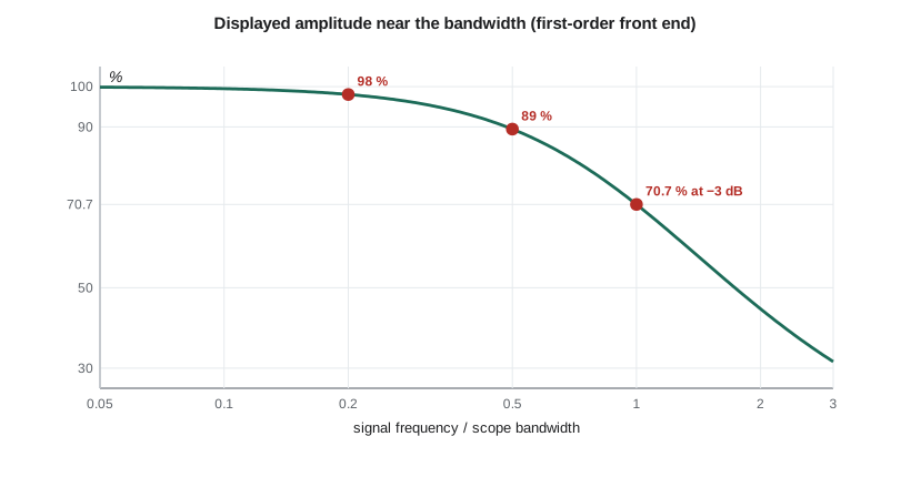
A scope's analog front end, probe and amplifier together, behaves like a low-pass filter. Its bandwidth is the frequency at which a sine wave's displayed amplitude has fallen by 3 dB, to about 70.7 % of its true value. A 100 MHz scope does not show 100 MHz sines at full height; it shows them about 30 % low. Even well below the bandwidth there is some loss: for a simple first-order response, a sine at half the bandwidth is displayed about 11 % low, and at one-fifth of the bandwidth about 2 % low. The common rule of thumb is to use a scope whose bandwidth is at least three to five times the highest frequency you need to measure accurately.

For edges, the useful relation links bandwidth to rise time. A system with a first-order or Gaussian-like response has a 10–90 % rise time of about 0.35 divided by its bandwidth: a 100 MHz scope has an intrinsic rise time of about 3.5 ns. When a signal with its own rise time passes through a scope, and through a probe with its own rise time, the displayed rise time is approximately the root-sum-square of all of them. That tells you how fast a scope must be to measure a given edge, and how to correct a measurement made with one that is not quite fast enough.

Sampling and aliasing

A digital scope's converter takes samples at a finite rate, and the sampling theorem from Signals and Systems applies: a signal can be represented faithfully only if it contains no frequencies above half the sample rate, the Nyquist frequency. Content above it folds back and appears at a false, lower frequency, an alias. A real-time scope samples fast enough that its own front-end bandwidth keeps the input below Nyquist, typically sampling at least 2.5 to 5 times its bandwidth. The danger comes when the timebase is slow: with shallow memory, a long time window forces a low sample rate, and a fast signal can alias into a slow-looking waveform that seems stable and plausible.

Two acquisition modes help. Peak-detect mode samples at the maximum rate internally and keeps the highest and lowest value in each display interval, so narrow glitches and high-frequency noise show up as a thick trace rather than as a misleading alias. High-resolution or averaging modes do the opposite: they combine adjacent fast samples, or successive triggered captures, to reduce noise and increase effective resolution at the cost of bandwidth. The bandwidth-limit switch, usually 20 MHz, inserts a filter that removes high-frequency noise you do not care about, which cleans up power-rail ripple measurements considerably.

Probe loading at high frequency

Lesson 6 described a 10X probe as 10 MΩ in parallel with about 10 to 15 pF. At DC the 10 MΩ dominates and the loading is tiny. At high frequency the capacitance dominates: 12 pF has a reactance of about 1.3 kΩ at 10 MHz and 130 Ω at 100 MHz. Probing a node with a source resistance of a few kilohms at those frequencies forms a low-pass filter that slows its edges, sometimes enough to make a marginal circuit fail only while you are probing it, or to make it work only while you are probing it. For fast, high-impedance signals, active probes with input capacitance below 1 pF, or low-impedance probes for 50 Ω systems, reduce the loading.

# Bandwidth, rise time, probe loading and alias frequency calculations
import math

def displayed_fraction(f, bw):          # first-order front end
    return 1 / math.sqrt(1 + (f / bw) ** 2)

for frac in (0.2, 0.33, 0.5, 1.0):
    print(f"sine at {frac:4.2f} x bandwidth displayed at {100*displayed_fraction(frac, 1):5.1f} %")

def true_rise(displayed_ns, scope_bw_mhz, probe_bw_mhz=None):
    parts = [(0.35 / scope_bw_mhz) * 1e3]
    if probe_bw_mhz: parts.append((0.35 / probe_bw_mhz) * 1e3)
    return math.sqrt(max(displayed_ns**2 - sum(p * p for p in parts), 0))

print(f"edge on 50 MHz scope:  {true_rise(8.0, 50):.2f} ns")
print(f"edge on 200 MHz scope: {true_rise(4.3, 200):.2f} ns")

# RC corner when a 12 pF probe loads a node with 4.7 kohm source resistance
R, C = 4.7e3, 12e-12
print(f"probe-loaded corner frequency: {1/(2*math.pi*R*C)/1e6:.2f} MHz, added rise time {2.2*R*C*1e9:.1f} ns")

def alias(f, fs):
    k = round(f / fs)
    return abs(f - k * fs)

for fs in (10e3, 100e3, 1e6, 10e6):
    print(f"fs = {fs/1e3:7.0f} kSa/s: 100.004 kHz appears at {alias(100004, fs):10.1f} Hz")

sine at 0.20 x bandwidth displayed at  98.1 %
sine at 0.33 x bandwidth displayed at  95.0 %
sine at 0.50 x bandwidth displayed at  89.4 %
sine at 1.00 x bandwidth displayed at  70.7 %
edge on 50 MHz scope:  3.87 ns
edge on 200 MHz scope: 3.93 ns
probe-loaded corner frequency: 2.82 MHz, added rise time 124.1 ns
fs =      10 kSa/s: 100.004 kHz appears at        4.0 Hz
fs =     100 kSa/s: 100.004 kHz appears at        4.0 Hz
fs =    1000 kSa/s: 100.004 kHz appears at   100004.0 Hz
fs =   10000 kSa/s: 100.004 kHz appears at   100004.0 Hz

The last section of the output is a practical test. At 10 kSa/s and at 100 kSa/s the regulator noise appears at 4 Hz, because 100.004 kHz sits just above a multiple of both sample rates; once the sample rate rises above twice 100 kHz, it appears at its true frequency. Real signals do not change frequency when you change the timebase; aliases do.

Grounding and the mains-referenced scope

On almost all bench oscilloscopes, the outer conductor of every input connector, and therefore every probe ground clip, is connected to the scope's chassis and through the power cord to the building's protective earth. A probe measures the voltage between its tip and earth, not between its tip and its ground clip. That is harmless when the circuit's ground is also at earth potential or floating, as with a battery-powered board or a board powered from an isolated bench supply. It is dangerous when you clip the ground lead to a point that is not at earth potential, such as the high side of a resistor, the switch node of a converter, or anything in a mains-connected, non-isolated circuit. The ground clip then shorts that point to earth through the probe, and the fault current flows through the probe's thin shield.

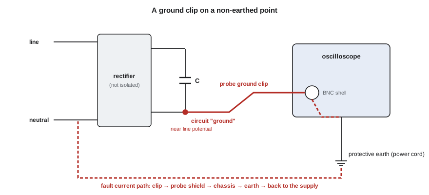
That is what happened on Leo's test fixture. The fixture's power supply rectifies mains directly, so its internal ground sits near line potential for half of each cycle. When he clipped the probe's ground there, the fault current tripped the breaker. He was lucky: the ground lead could have burned open and the scope's input could have been damaged. The correct ways to measure such points are a differential probe, which measures the voltage between two points without connecting either to earth; an isolated-input scope or a battery-powered handheld scope rated for the measurement category; or two channels in the scope's math mode, subtracting one from the other, which works for slow signals with small common-mode voltages. Defeating the scope's earth with a cheater plug is never acceptable; it puts the chassis and every exposed metal part at the circuit's voltage.

Grounding also causes noise even when nothing is shorted. If the circuit under test is earthed at one point, through its supply, and the scope is earthed at another, through its cord, the probe ground lead closes a ground loop. Small voltage differences between the two earth points drive current around the loop, and the loop picks up magnetic fields from nearby wiring. The result is often a 60 Hz hum or spiky noise on the trace that is not in the circuit. Keeping the probe ground lead short, using a single ground point for the setup, and powering the circuit from a floating supply all reduce it.

The frequency domain: the scope's FFT

Most digital scopes can display a fast Fourier transform of the captured waveform, showing amplitude against frequency instead of against time. It is the quickest way to answer questions such as which harmonics are in the LED driver's switching current, where the noise on a sensor line comes from, or whether a filter is removing what it should. The FFT's frequency resolution is the sample rate divided by the number of points, so a longer capture gives finer resolution. Its span reaches half the sample rate. A window function, such as Hann or flat-top, reduces the leakage of a strong component into neighboring bins at the cost of slightly wider peaks. The vertical axis is usually in dBV or dBm, which makes small components visible next to large ones.