Code generation and register allocation

The back end turns optimized IR into machine code. It has three classic tasks. Instruction selection chooses machine instructions to implement each IR operation, exploiting the target's addressing modes and specialized instructions. Register allocation maps the unlimited virtual registers or temporaries of the IR onto the handful of physical registers the processor has, storing values in memory, spilling them, when registers run out. Instruction scheduling orders instructions to keep the processor's pipeline busy. Each task is hard in general: optimal instruction selection for DAGs, optimal register allocation and optimal scheduling are all NP-complete problems, so back ends use well-engineered heuristics. This lesson targets RISC-V, which CMPUT-229 used, though the techniques are those of every production back end.

Instruction selection as tree tiling

After lowering, each basic block can be viewed as a forest of expression trees, with nodes for operations such as add, multiply, load and constants. Each machine instruction corresponds to a small tree pattern, a tile: an add instruction covers one + node with two register operands; RISC-V's addi covers a + node whose right operand is a 12-bit constant; a load lw rd, off(rs) covers a load node whose address is a register plus a small constant, taking three IR nodes in one instruction. Instruction selection is the problem of covering the tree with tiles so that every node is covered exactly once and tiles connect at their roots and leaves, at minimum total cost. Simple RISC instruction sets have few interesting tiles; complex ones such as x86-64, with memory operands and scaled-index addressing, have many.

Two algorithms dominate. Maximal munch, a greedy top-down method, starts at the root, picks the largest tile that matches there, and recursively tiles the subtrees left uncovered. It produces an optimal tiling in the sense that no two adjacent tiles could be combined into a larger one, though not necessarily the minimum-cost tiling. Dynamic programming, as in the code generator generators BURG and iburg (Christopher Fraser, David Hanson and Todd Proebsting, early 1990s), computes bottom-up the minimum-cost tiling of every subtree for every kind of result and gives a truly optimal tiling for trees. LLVM's SelectionDAG instruction selector matches patterns written in its TableGen description language over a DAG per basic block, and its newer GlobalISel framework selects instructions over whole functions; GCC matches RTL patterns from its machine description files.

# Instruction selection by maximal munch over expression trees, for a
# RISC-V-like target. Larger tiles (addi with an immediate, a load with an
# offset, slli for multiplying by a power of two) are tried before small ones.
# Tree nodes: ("+", a, b), ("*", a, b), ("load", addr), ("const", n), ("reg", name)
from itertools import count
regs = (f"v{i}" for i in count(1))                 # unlimited virtual registers
def munch(t, code):
    op = t[0]
    if op == "reg": return t[1]
    if op == "const":
        r = next(regs); code.append(f"li    {r}, {t[1]}"); return r
    if op == "load":
        a = t[1]                                     # tile: load with base + 12-bit offset
        if a[0] == "+" and a[2][0] == "const" and -2048 <= a[2][1] < 2048:
            base = munch(a[1], code); r = next(regs)
            code.append(f"lw    {r}, {a[2][1]}({base})"); return r
        base = munch(a, code); r = next(regs); code.append(f"lw    {r}, 0({base})"); return r
    if op == "+":
        for x, y in ((t[1], t[2]), (t[2], t[1])):    # tile: addi when one side is a small constant
            if y[0] == "const" and -2048 <= y[1] < 2048:
                s = munch(x, code); r = next(regs); code.append(f"addi  {r}, {s}, {y[1]}"); return r
        a, b = munch(t[1], code), munch(t[2], code); r = next(regs)
        code.append(f"add   {r}, {a}, {b}"); return r
    if op == "*":
        for x, y in ((t[1], t[2]), (t[2], t[1])):    # tile: shift for a power of two
            if y[0] == "const" and y[1] > 0 and y[1] & (y[1] - 1) == 0:
                s = munch(x, code); r = next(regs)
                code.append(f"slli  {r}, {s}, {y[1].bit_length() - 1}"); return r
        a, b = munch(t[1], code), munch(t[2], code); r = next(regs)
        code.append(f"mul   {r}, {a}, {b}"); return r
def naive(t, code):                                  # one instruction per node, no big tiles
    op = t[0]
    if op == "reg": return t[1]
    r = next(regs)
    if op == "const": code.append(f"li    {r}, {t[1]}"); return r
    if op == "load": a = naive(t[1], code); code.append(f"lw    {r}, 0({a})"); return r
    a, b = naive(t[1], code), naive(t[2], code)
    code.append(f"{'add ' if op == '+' else 'mul '}  {r}, {a}, {b}"); return r
# x = a[i] + p.f, where a is an int array in register a0, i is in a1, and the
# struct pointer p is in a2 with field f at offset 8
tree = ("+", ("load", ("+", ("reg", "a0"), ("*", ("reg", "a1"), ("const", 4)))),
             ("load", ("+", ("reg", "a2"), ("const", 8))))
for name, sel in (("maximal munch", munch), ("one node per instruction", naive)):
    regs = (f"v{i}" for i in count(1)); code = []
    result = sel(tree, code)
    print(f"{name}: {len(code)} instructions, result in {result}")
    for c in code: print("    " + c)

maximal munch: 5 instructions, result in v5
    slli  v1, a1, 2
    add   v2, a0, v1
    lw    v3, 0(v2)
    lw    v4, 8(a2)
    add   v5, v3, v4
one node per instruction: 8 instructions, result in v1
    li    v5, 4
    mul   v4, a1, v5
    add   v3, a0, v4
    lw    v2, 0(v3)
    li    v8, 8
    add   v7, a2, v8
    lw    v6, 0(v7)
    add   v1, v2, v6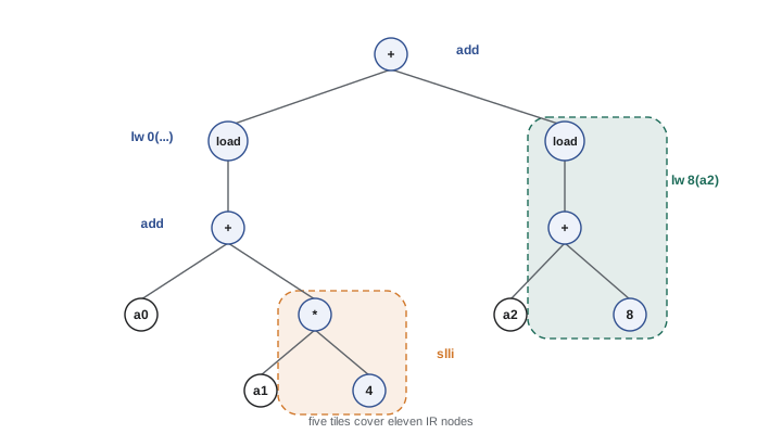

The larger tiles make a real difference: multiplying by 4 becomes a shift, and the field access p.f becomes a single load with an offset, so maximal munch needs 5 instructions where the naive translation needs 8, two of them just to load the constants 4 and 8 into registers. On x86-64, the whole address a + i × 4 would fit inside a single load's addressing mode. Real selectors also handle conditional branches by fusing a comparison with the branch that uses it (RISC-V's blt rs1, rs2, label tests and branches in one instruction), and recognize idioms such as fused multiply-add, bit-field extraction and rotates.

Register allocation: the problem

Registers are the fastest storage in a computer, and there are few of them: RISC-V has 31 usable integer registers, of which a function can freely use around 25 after accounting for the stack pointer, return address and other reserved roles; x86-64 has 16. The IR, by contrast, uses as many temporaries as it likes. The register allocator must decide which values live in registers at each point, and when there are not enough, which to keep in memory. A good allocation can easily double the speed of a loop compared with a poor one. Two values can share a register only if they are never needed at the same time, so the allocator needs to know when each value is needed: its live range, computed by liveness analysis.

A variable is live at a point if its current value may be used later along some path before being overwritten. Liveness is a backward data-flow problem: working backward through a block, the variables live before an instruction are those it uses plus those live after it, minus the one it defines. Across a CFG, the variables live at the end of a block are those live at the start of any successor, iterated to a fixed point; lesson 11 develops this general framework. Two variables interfere if one is live at the point where the other is defined; interfering variables need different registers.

Graph coloring

Gregory Chaitin and colleagues at IBM (1981 to 1982) turned register allocation into graph coloring. The interference graph has a node per variable and an edge between interfering variables; assigning K registers is coloring the graph with K colors so that adjacent nodes differ. Graph coloring is NP-complete, but Chaitin's heuristic works well. Its key observation: a node with fewer than K neighbors can always be colored, whatever colors its neighbors get. So the allocator repeatedly removes such a node from the graph and pushes it on a stack, simplifying the graph; then it pops nodes one by one, giving each a color unused by its already-colored neighbors. If at some point every remaining node has K or more neighbors, a node is chosen to spill, ideally one with many neighbors and few uses, weighted by loop depth.

Preston Briggs, Keith Cooper and Linda Torczon (1989 to 1994) improved this with optimistic coloring. Instead of spilling immediately when simplification gets stuck, the allocator pushes a spill candidate on the stack anyway and continues; when it is popped, its neighbors may happen to use fewer than K colors, in which case it gets a register after all. Only nodes that truly find no free color are spilled. Spilling a variable means storing it to a stack slot after each definition and loading it before each use, which splits its long live range into tiny ones; the allocator then rebuilds the graph and tries again.

# Register allocation by assigning K registers to a graph (Chaitin-Briggs): liveness analysis,
# the interference graph, simplify with optimistic spilling, then select.
# Straight-line code from a loop body, with the registers live on exit.
CODE = [("a", ["x"]), ("b", ["x", "y"]), ("c", ["a", "y"]), ("d", ["a", "b"]),
        ("e", ["c", "d"]), ("f", ["b", "e"]), ("g", ["e", "f", "c"]), ("h", ["g", "d"])]
LIVE_OUT = {"h", "f"}
# 1. Liveness, computed backwards: live_before = uses U (live_after - def)
live, after = set(LIVE_OUT), []
for d, uses in reversed(CODE):
    after.append(set(live)); live = (live - {d}) | set(uses)
after.reverse()
print("live into the block:", sorted(live))
# 2. Interference: a definition interferes with everything live after it
nodes = {d for d, _ in CODE} | {"x", "y"}
adj = {n: set() for n in nodes}
for (d, _), out in zip(CODE, after):
    for v in out - {d}: adj[d].add(v); adj[v].add(d)
for v in live:                                        # values live on entry interfere pairwise
    adj[v] |= live - {v}
print("interference degrees:", {n: len(adj[n]) for n in sorted(nodes)})
def allocate(K):
    work, stack, g = set(nodes), [], {n: set(adj[n]) for n in nodes}
    while work:
        low = sorted(n for n in work if len(g[n] & work) < K)
        n = low[0] if low else max(sorted(work), key=lambda m: len(g[m] & work))   # optimistic spill candidate
        stack.append((n, not low)); work.remove(n)
    reg, spilled = {}, []
    while stack:
        n, candidate = stack.pop()
        used = {reg[m] for m in adj[n] if m in reg}
        free = [r for r in range(K) if r not in used]
        if free: reg[n] = free[0]
        else: spilled.append(n)
    return reg, spilled
for K in (4, 3):
    reg, spilled = allocate(K)
    names = [f"s{i + 1}" for i in range(K)]
    assigned = ", ".join(f"{n}->{names[reg[n]]}" for n in sorted(reg))
    print(f"K={K}: {assigned}" + (f"   spilled: {spilled}" if spilled else "   (no spills)"))

live into the block: ['x', 'y']
interference degrees: {'a': 4, 'b': 5, 'c': 5, 'd': 5, 'e': 4, 'f': 5, 'g': 2, 'h': 1, 'x': 2, 'y': 3}
K=4: a->s3, b->s2, c->s4, d->s3, e->s1, f->s2, g->s1, h->s1, x->s2, y->s1   (no spills)
K=3: a->s2, b->s1, d->s3, e->s2, f->s1, g->s2, h->s2, x->s1, y->s3   spilled: ['c']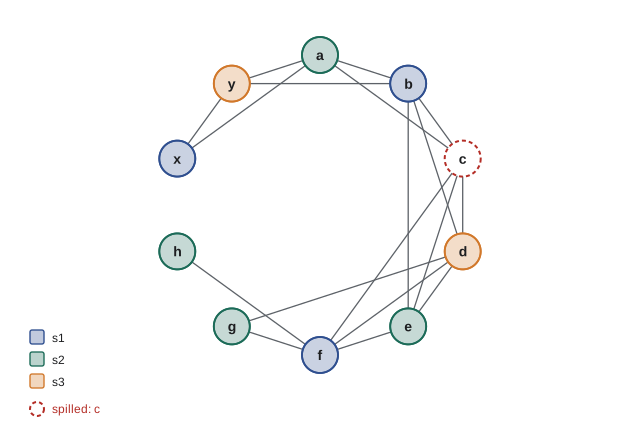

With four registers every value fits. With three, the coloring gets stuck and one value, c, is spilled to memory: it is live across the definitions of d, e and f while a, b or their successors also need registers. Because the allocator is optimistic, it spills only the value that genuinely found no free color after its neighbors were colored, not every candidate it was unsure about. In a full compiler the spilled value would get a frame slot (lesson 9), and the allocator would insert the loads and stores and repeat.

Coalescing and pre-coloring

Two refinements matter in practice. Copy instructions such as x = y, which arise from φ removal (lesson 8), from calling conventions and from the IR generator, are free if x and y share a register. Coalescing merges the nodes of a copy's source and destination when they do not interfere, deleting the copy. Coalescing too aggressively can make the graph impossible to color with K registers, so allocators use conservative tests, such as Briggs's: merge only if the combined node would have fewer than K neighbors of significant degree. Lal George and Andrew Appel's iterated register coalescing (1996) interleaves simplification and conservative coalescing and is the standard textbook allocator. Pre-colored nodes represent physical registers with fixed roles: arguments must arrive in a0 to a7, results leave in a0, and a call destroys every caller-saved register, which the allocator models by making values live across a call interfere with all caller-saved registers, steering them into callee-saved ones.

Linear scan

Graph coloring is too slow for some settings, notably JIT compilers, where compile time is part of the program's running time. Massimiliano Poletto and Vivek Sarkar's linear scan allocator (1999) approximates each variable's live range by a single interval, from its first definition to its last use in a linear order of the code, then sweeps the intervals in order of their start points. It keeps the currently active intervals; when one ends, its register is freed; when a new interval starts and no register is free, it spills whichever active interval ends last, freeing a register for the longest time. Linear scan runs in nearly linear time and produces code only a little worse than coloring. Refinements that split intervals and fill holes in live ranges, such as the second-chance binpacking and the HotSpot client compiler's allocator by Christian Wimmer and Hanspeter Mössenböck (2005), are used in HotSpot, V8 and other JITs; LLVM's default greedy allocator is a priority-based hybrid that splits live ranges aggressively.

# Linear-scan register allocation (Poletto and Sarkar, 1999): sort live
# intervals by start, keep the active ones sorted by end, and when no register
# is free spill the interval that ends last. Used by many JIT compilers.
intervals = {"a": (1, 4), "b": (2, 6), "c": (3, 5), "d": (4, 8), "e": (5, 7),
             "f": (6, 9), "g": (7, 8), "h": (8, 9)}            # (first def, last use)
def linear_scan(K):
    free, active, where = [f"r{i}" for i in range(K)], [], {}
    for v, (start, end) in sorted(intervals.items(), key=lambda kv: kv[1][0]):
        for w in [w for w in active if intervals[w][1] <= start]:   # expire old intervals
            active.remove(w); free.append(where[w])
        if free:
            where[v] = free.pop(0); active.append(v)
        else:
            victim = max(active, key=lambda w: intervals[w][1])
            if intervals[victim][1] > end:                         # steal from the longest
                where[v] = where[victim]; where[victim] = "stack"
                active.remove(victim); active.append(v)
            else: where[v] = "stack"
        active.sort(key=lambda w: intervals[w][1])
    return where
for K in (3, 2):
    w = linear_scan(K)
    print(f"K={K}:", ", ".join(f"{v}->{w[v]}" for v in sorted(w)),
          f"| spilled: {[v for v in w if w[v] == 'stack'] or 'none'}")

K=3: a->r0, b->r1, c->r2, d->r0, e->r2, f->r1, g->r2, h->r0 | spilled: none
K=2: a->r0, b->stack, c->r1, d->r0, e->r1, f->stack, g->r1, h->r0 | spilled: ['b', 'f']

Instruction scheduling

Modern processors overlap the execution of instructions in a pipeline, and an instruction that needs a result not yet available stalls. A load that misses in the first-level cache, or a multiply, may take several cycles. Instruction scheduling reorders independent instructions so that useful work fills those cycles. List scheduling, the standard algorithm, builds the dependence DAG of a basic block, assigns each instruction a priority such as the length of the longest path from it to the end, and fills each cycle with the highest-priority instruction whose operands are ready. Scheduling and register allocation interact: scheduling for parallelism lengthens live ranges and increases register pressure, while allocation introduces false dependences between unrelated values that happen to share a register. Compilers often schedule both before and after allocation. Out-of-order processors, which reorder instructions in hardware, reduce the benefit of static scheduling but do not eliminate it, and for in-order cores, common in embedded RISC-V designs, it matters greatly. Software pipelining applies scheduling across loop iterations, overlapping the start of one iteration with the end of the previous.

Emitting code

The last step writes assembly language or, more often today, object code directly. It lays out basic blocks, ideally so that the most frequent successor follows its predecessor and needs no jump; resolves branch targets and chooses short or long branch forms; emits constants and data; and produces symbols, relocations and debugging information for the linker (CMPUT-229 lesson 8 follows this path into linking and loading). Peephole optimization, examining a small sliding window of instructions and replacing patterns with cheaper equivalents, cleans up local inefficiencies such as a store immediately followed by a load from the same location, or a jump to the next instruction.

Worked examples